Logistic Regression
Python implementation of the Logistic Regression model, applied to and analysed on the iris dataset and the monk dataset. Main implementation of the algorithm can be found in src/logistic.py. A theoretical description of the model and the implementation is given below.
Requirements
Required packages are listed in requirements.txt. Install them into your virtual environment with
pip install -r requirements.txt
Usage
usage: evaluate.py [-h] [--dataset {iris,monk}]
               [--features {0,1,2,3} [{0,1,2,3} ...]] [--exploration]
               [--performance] [--decision-boundary] [--no-plot] [--safe]

optional arguments:
  -h, --help            show this help message and exit
  --dataset {iris,monk}
                        the dataset to be used, either iris or monk
  --features {0,1,2,3} [{0,1,2,3} ...]
                        features used when dataset is iris
  --exploration         whether to plot the pairplot
  --performance         whether to plot performance measures
  --decision-boundary   whether to plot/save the decision boundary
  --no-plot             deactivate plotting for the decision boundary
  --safe                activate saving of decision boundary plot
Model
The logistic regression model for binary classification is single-layered and has only one output unit that models the probability over the binary output by a Bernoulli distribution. The number of input units is determined by the number of features in the dataset, but augmented by one neuron of constant value 1 to represent the bias. A forward pass through this model is hence performed by the following equation:
That is, we take the dot product (sum of element-wise products) of weights (plus bias) and the augmented input
and squeeze it into the range
using the sigmoid function
.
To update , we employ the Gradient Descent algorithm with batch size 1, i.e., Stochastic Gradient Descent (SGD). Thus, during training, at each step the model samples one instance from the dataset without replacement. It then performs the forward pass to make a prediction
. The objective of logistic regression is the maximization of the log likelihood of true labels
given data
and parameters
. We can maximize by minimizing its negation using Gradient Descent. The gradient of the logistic loss for weight
is given by
Based on the prediction from the forward pass, the true label
and the input feature
, SGD then updates the weights using the delta rule
The negation of is necessary since we minimize in gradient descent, but want to maximize the log likelihood (and therefore minimize its negation).
is the learning rate that controls the step size of the Gradient Descent. If steps are too small, learning will take too long. If the steps are too large, it can happen that the optimization does not converge to the minimum but oscillates around it.
Furthermore, a regularization term is added to the loss , controlled by the weight decay rate
:
The partial derivative that needs to be added to the gradient of equation [eq:gradient] is
Since we do not want to prevent the bias from taking any necessary value, we only apply weight decay to all except for
.
Data
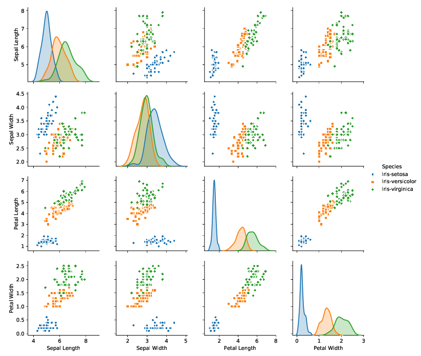
The logistic regression model described above is tested on two datasets: the iris dataset and the monk dataset. The iris dataset consists of three classes, with 50 data points each. The figure above visualizes the dataset in a pairplot. It becomes apparent from this plot that the classes setosa and versicolor can be unambigously distinguished by the use of any two features. We will leverage this fact in order to make the above described model applicable to the iris dataset by only taking the first 100 samples into account and hence dropping the last class. The clear distinguishability of the remaining classes allows us to experiment with only 2 input features that we can plot along the learned decision boundary.
The monk dataset is an artificial dataset consisting of 2 classes. It can therefore be used out of the box for this model. There are a total of 432 samples with 6 features, all in the form of integers.
Preprocessing
As both iris and monk are presented in convenient format, not much preprocessing is necessary. In fact, we only apply normalization of the features by using z-score standardization given as
where is the mean and
the standard deviation of the
feature. For both datasets, the samples are randomly distributed over
train and test set in a 80/20 split.
Results
Iris Dataset
For experiments on the Iris dataset, the learning rate is set to
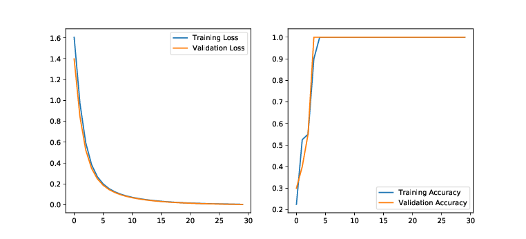
0.05 and the weight decay to 0.005. The figure above shows the development of loss and accuracy over epochs of
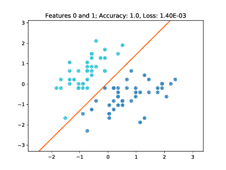
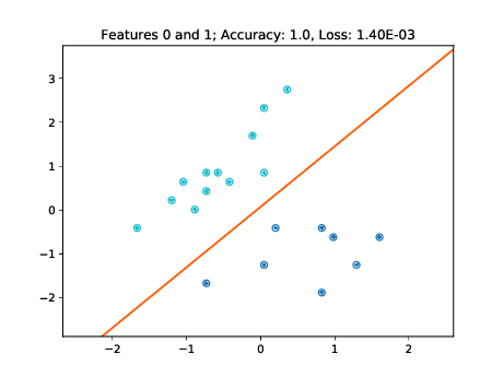
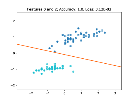
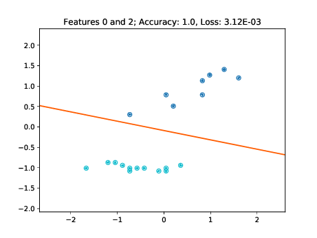
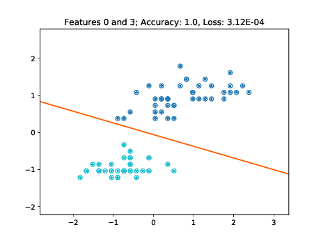
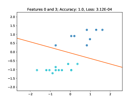
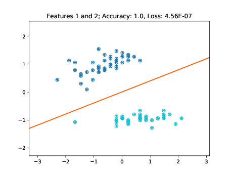
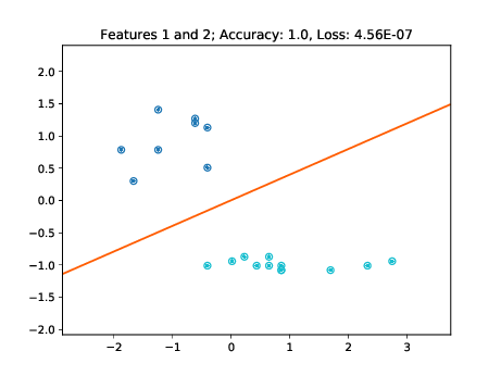
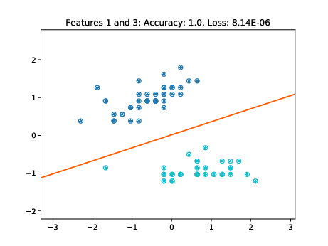
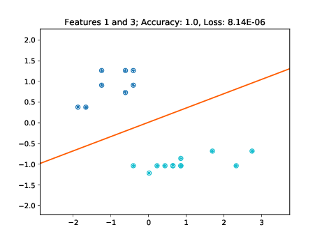
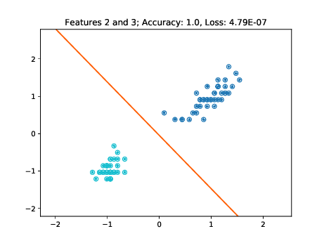
training. The figures below show
the decision boundaries trained with different feature pairs along the
training and testing data points respectively.
| Train Data | Test Data |
|---|---|
 |
 |
 |
 |
 |
 |
 |
 |
 |
 |
 |
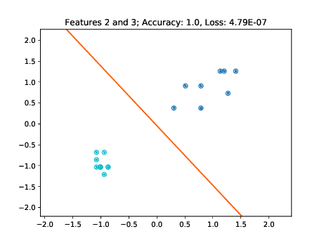 |
As these figures demonstrate, the learned decision boundaries separate the two clusters of points corresponding to two classes without errors. The decision boundaries also work for the unseen test data. Note though, that for example in the two bottom left plots of Figure [fig:decision-boundaries] there are some data points lying further away from the cluster. If these would have not been part of the training set, then the decision boundary may have been further tilted in a way minimizing the loss of the training data, but misclassifying these "outliers" in the test set.
Effect of Regularization
Table 1 shows results on the iris dataset (using features 0 and 2) after
200 epochs for three configurations: no regularization at all,
regularization with and regularization with
. Only the loss is reported as the accuracy stays at
and does not allow for nuanced analysis. With a low
both the train and test loss decrease. With a higher
weight decay of
, the test loss[1] further decreases
while the train loss increases. While the model is still very good for
the test data, we hence observe first signs of underfitting due to too
much regularization. These results were consistent using different
random seedings.
| Train | Test | |
|---|---|---|
| No Regularization | 0.032 | 0.0173 |
| 0.005 | 0.0218 | 0.0079 |
| 0.05 | 0.3568 | 0 |
Loss after 200 epochs on the iris dataset using no regularization,
weight decay with rate and rate
.
Learning Rate Tuning
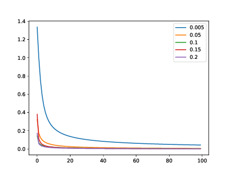
We can explore the effects of different learning rates by
plotting the convergence of the model when using them. Such a plot is
given in the figure above. It can be clearly observed, that lower
learning rates cause slower convergence, but for this simple problem do
not results in better convergence at later epochs. Given the very low
loss achieved after only few epochs when using higher learning rates
such as
shows that the simplicity of the problem allows for
choosing such high learning rates.
Monk Dataset
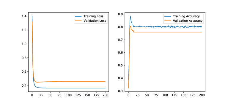
The monk data set turned out to be a more complicated problem and the
model did not manage to achieve accuracy. Figure
4 shows the development of loss and accuracy. As a
learning rate,
showed to produce good results based on
informal experiments. A weight decay actually showed to be harmful in
this experiment, which is why it is deactivated here. Table
[tab:monk] also shows exact results on the monk dataset
after
epochs.
| Train | Test | |
|---|---|---|
| Accuracy | 0.758 | 0.8 |
| Loss | 0.457 | 0.36 |
Loss and Accuracy after 200 epochs on the monk dataset.
