Grender-classification-Artificial-Neural-Nets
This classifiers the gender of the person speaking in the singular audio file using Artificial Neural Networks
Audio
Male/Female
Project Structure
steps
1.Introduction and Papers.
2.Approches
3.Data collection and Preprocessing
4.signal Transformation
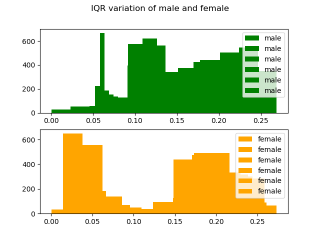
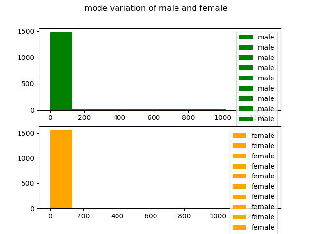
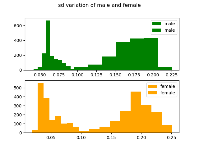
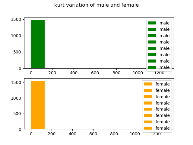
5.Feature Extraction and visualisation
6.Training
7.Testing
8.Evaluation
9.Output
10.References
1. Introduction
This project uses a mathamatical approach to determine the gender of the person speaking in the audio file .the implementation focusses more on the audio that consist the voice of a single person speaking at a time.As we know that directly we cannot use the audio data because it may consist some noise and other factors that we may not want to use.
To make our work easier we will be using the algorithm called Fast Fourier Transformation (FFT) . this technique will help us to extract better quality of features and those features will be using to train the classification model using Deep Neural Networks method called Artificial Neural Networks
Papers
The papers which we will be going to focus more are :
1.Gender Classification in Speech Recognition using Fuzzy Logic and Neural Network # 3rd paper in the papers dataset
2.Musical Genre Classification of Audio Signals # 4th paper from the IEEE Papers dataset
2.Approches
The steps that we are going to take to build the model are as follows:
1. Load the audio file.
2. Transform the audio signal using FFT.
3. Extract meaningful features.
4. create the dataset.
5. cleaning the dataset.
6. scaling the dataset.
7. Building Neural Nets.
8. Training the model.
9. Accuracy calculation.
10.Performance tuning.
11.Deploying the Model.
3.Data collection and Preprocessing
I have uploaded the dataset that i used in the dataset forlder which contains two types of data.The first type of data is the actual audio data nad the second type of data is the the csv data whch contains the extracted features from real audio data. I will be shuffleing both the data after extraction of features.
4.Signal Transformation
Initially the data dataset contains all the audio files, so we need to transform each audio file in the folder using FFT .
FFT IMPLEMENTATION IN PYTHON3
	#defining omega for FFT
	@classmethod
	def omega(self,p, q):
		return cmath.exp((2.0 * cmath.pi * 1j * q) / p)

	#actual defination for Fast fourier Transformation (FFT)
	@classmethod
	def fft(self,signal):

		#length of the signal
		n = len(signal)
		if n == 1:
			return signal
		else:
			#splitting into even and odd set
			Feven = self.fft([signal[i] for i in range(0, n, 2)])
			Fodd = self.fft([signal[i] for i in range(1, n, 2)])


		combined = [0] * n #combining the both list
		for m in range(n//2):
			combined[m] = Feven[m] + self.omega(n, -m) * Fodd[m]
			combined[m + n//2] = Feven[m] - self.omega(n, -m) * Fodd[m]

		#returning while converting list to numpy array
		return np.array(combined)
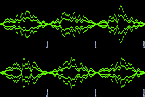
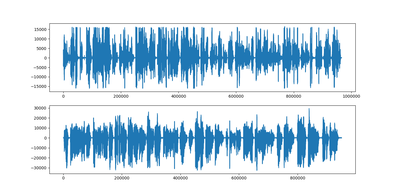
sample audio plotting :
Male vs Female
Male vs Female
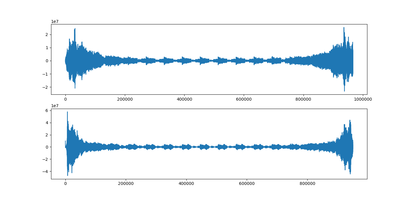
sample audio plotting after transformation:
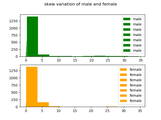
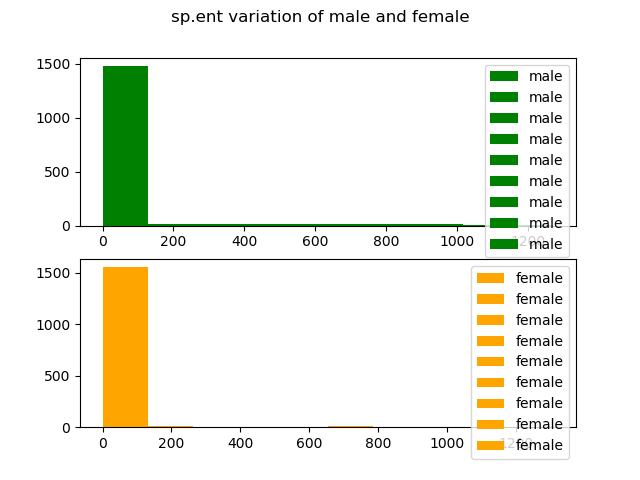
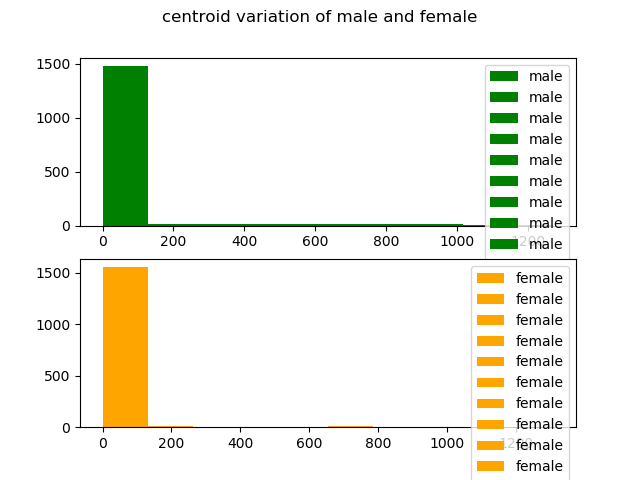
5.Feature Extraction and visualisation
The List of MFCC Features which i will be using are as follows :
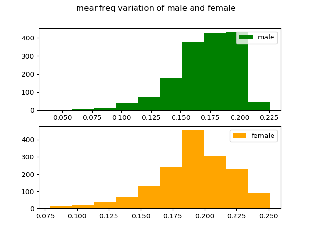
1.Mean Frequency
2.Standard Devation
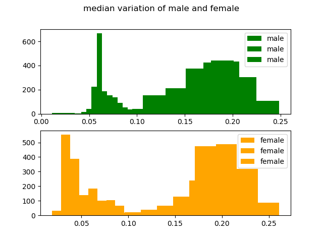
3.Median
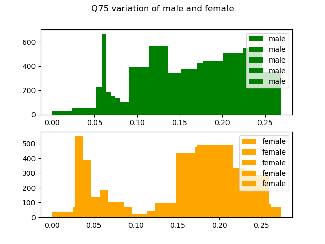
4.Third Quartile (Q75)
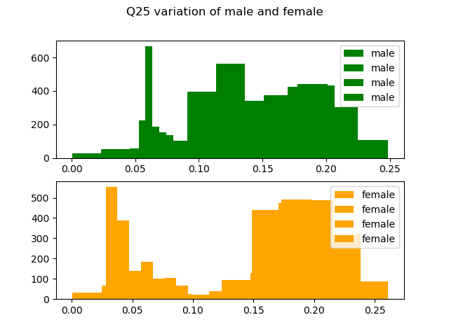
5.First Quartile(Q25)
6.Inter Quartile(IQR)
7.Skewness
8.Kurtosis
9.Spectral Entropy
10.Spectral Flatness
11.Mode
12.Central Frequency


Q.What is MFCC ?

Ans:-Mel-frequency cepstral coefficients (MFCCs) are coefficients that collectively make up an MFC.
They are derived from a type of cepstral representation of the audio clip (a nonlinear "spectrum-of-
a-spectrum").
References Used :
“The International Arab Journal of Information Technology, Vol. 10, No. 5, September 2013”
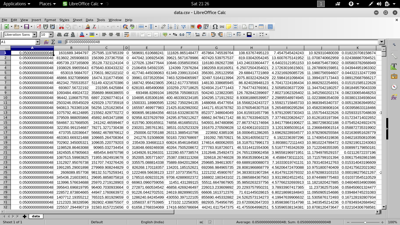
Dataset Snapshot
Extracted Feature
Visualization
6. Training
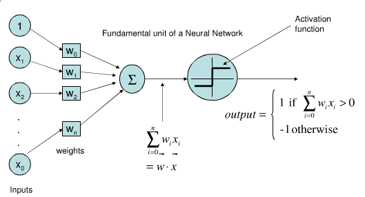
Using Artifcial Neural Network to train the model for classification problem because Neural Nets seems to give the most accurate results in terms of accuracy.
The description of the architecture i am using for classification are as follows:
1. 1 input layer , Hidden layer, 1 Output Layer.
2. using 12 input attributes and 1 output attributes.
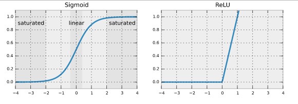
3. activation function for input and hidden layer is “relu”.
4. activation function for output layer is “sigmoid”.
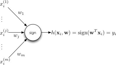
5. using 10 perceptron in each input and hidden layer.
6. for optimisation algorthm is used “adam”.
Q. What is Perceptron?
Ans :
a computer model or computerized machine devised to represent or simulate the ability of the brain to recognize and discriminate.
Q.What is activation Function?Ans :
In artificial neural networks, the activation function of a node defines the output of that node given an input or set of inputs. A standard computer chip circuit can be seen as a digital network of activation functions that can be "ON" (1) or "OFF" (0), depending on input.
ReLu activation Function:
A unit employing the rectifier is also called a rectified linear unit (ReLU). A smooth approximation to the rectifier is the analytic function
F(x) = Log(1 + exp(x))
which is called the softplus function
Sigmoid activaton Function:
It is used in neural networks to give logistic neurons real-valued output that is a smooth and bounded function of their total input. It also has the added benefit of having nice derivatives which make learning the weights of a neural network easier.
F(x) = 1/ (1 + exp(-x))
Graphical Representation
Implementation
Modules used:
import numpy as np
import pandas as pd
import h5py
from sklearn.model_selection import train_test_split
from keras.models import load_model
from keras.models import Sequential
from keras.layers import Dense, Dropout
from keras import optimizers
from sklearn.utils import shuffle
import matplotlib.pyplot as plt
from sklearn.metrics import confusion_matrix
Using python keras module for layer creation and compilation:
# Initialising the ANN
classifier = Sequential()

# Adding the input layer and the first hidden layer
classifier.add(Dense(output_dim = 10, init = 'uniform', activation = 'relu', input_dim = 12))

# Adding the second hidden layer
classifier.add(Dense(output_dim = 10, init = 'uniform', activation = 'relu'))

# Adding the third hidden layer
classifier.add(Dense(output_dim = 10, init = 'uniform', activation = 'relu'))

# Adding the output layer
classifier.add(Dense(output_dim = 1, init = 'uniform', activation = 'sigmoid'))

# Compiling the ANN
classifier.compile(optimizer = 'adam', loss = 'binary_crossentropy', metrics = ['accuracy'])

# Fitting the ANN to the Training set
history = classifier.fit(x_train, y_train, batch_size = 20, nb_epoch = 200)
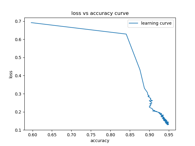
Learnng Curve:
Trainng process:
Epoch 1/200 2018-06-17 00:32:26.187508: I tensorflow/core/platform/cpu_feature_guard.cc:137] Your CPU supports instructions that this TensorFlow binary was not compiled to use: SSE4.1 SSE4.2 AVX AVX2 FMA 2121/2121 [==============================] - 2s 758us/step - loss: 0.6931 - acc: 0.5158 Epoch 2/200 2121/2121 [==============================] - 0s 186us/step - loss: 0.6824 - acc: 0.6587 Epoch 3/200 2121/2121 [==============================] - 0s 188us/step - loss: 0.6268 - acc: 0.7775 Epoch 4/200 2121/2121 [==============================] - 0s 184us/step - loss: 0.5613 - acc: 0.8345 Epoch 5/200 2121/2121 [==============================] - 0s 188us/step - loss: 0.4890 - acc: 0.8609 Epoch 6/200 2121/2121 [==============================] - 0s 188us/step - loss: 0.4284 - acc: 0.8779 Epoch 7/200 2121/2121 [==============================] - 0s 187us/step - loss: 0.3863 - acc: 0.8821 Epoch 8/200 2121/2121 [==============================] - 0s 189us/step - loss: 0.3598 - acc: 0.8883 Epoch 9/200 2121/2121 [==============================] - 0s 185us/step - loss: 0.3422 - acc: 0.8925 Epoch 10/200 2121/2121 [==============================] - 0s 189us/step - loss: 0.3334 - acc: 0.8949 Epoch 11/200 2121/2121 [==============================] - 0s 189us/step - loss: 0.3231 - acc: 0.8949 Epoch 12/200 2121/2121 [==============================] - 0s 191us/step - loss: 0.3145 - acc: 0.8986 Epoch 13/200 2121/2121 [==============================] - 0s 189us/step - loss: 0.3079 - acc: 0.8996 Epoch 14/200 2121/2121 [==============================] - 0s 190us/step - loss: 0.3035 - acc: 0.9005 Epoch 15/200 2121/2121 [==============================] - 0s 192us/step - loss: 0.2990 - acc: 0.9015 Epoch 16/200 2121/2121 [==============================] - 0s 188us/step - loss: 0.2944 - acc: 0.9010 Epoch 17/200 2121/2121 [==============================] - 0s 188us/step - loss: 0.2920 - acc: 0.9015 Epoch 18/200 2121/2121 [==============================] - 0s 191us/step - loss: 0.2878 - acc: 0.9019 Epoch 19/200 2121/2121 [==============================] - 0s 186us/step - loss: 0.2881 - acc: 0.8991 Epoch 20/200 2121/2121 [==============================] - 0s 190us/step - loss: 0.2831 - acc: 0.9029 Epoch 21/200 2121/2121 [==============================] - 0s 191us/step - loss: 0.2815 - acc: 0.9048 Epoch 22/200 2121/2121 [==============================] - 0s 188us/step - loss: 0.2765 - acc: 0.9024 Epoch 23/200 2121/2121 [==============================] - 0s 189us/step - loss: 0.2732 - acc: 0.9038 Epoch 24/200 2121/2121 [==============================] - 0s 189us/step - loss: 0.2708 - acc: 0.9033 Epoch 25/200 2121/2121 [==============================] - 0s 190us/step - loss: 0.2668 - acc: 0.9019 Epoch 26/200 2121/2121 [==============================] - 0s 188us/step - loss: 0.2621 - acc: 0.9033 Epoch 27/200 2121/2121 [==============================] - 0s 187us/step - loss: 0.2559 - acc: 0.9043 Epoch 28/200 2121/2121 [==============================] - 0s 192us/step - loss: 0.2467 - acc: 0.8986 Epoch 29/200 2121/2121 [==============================] - 0s 189us/step - loss: 0.2264 - acc: 0.9052 Epoch 30/200 2121/2121 [==============================] - 0s 193us/step - loss: 0.2173 - acc: 0.9104 Epoch 31/200 2121/2121 [==============================] - 0s 189us/step - loss: 0.2239 - acc: 0.9066 Epoch 32/200 2121/2121 [==============================] - 0s 188us/step - loss: 0.2056 - acc: 0.9175 Epoch 33/200 2121/2121 [==============================] - 0s 187us/step - loss: 0.2006 - acc: 0.9236 Epoch 34/200 2121/2121 [==============================] - 0s 190us/step - loss: 0.1979 - acc: 0.9236 Epoch 35/200 2121/2121 [==============================] - 0s 191us/step - loss: 0.1970 - acc: 0.9255 Epoch 36/200 2121/2121 [==============================] - 0s 189us/step - loss: 0.1932 - acc: 0.9260 Epoch 37/200 2121/2121 [==============================] - 0s 189us/step - loss: 0.1917 - acc: 0.9274 Epoch 38/200 2121/2121 [==============================] - 0s 187us/step - loss: 0.1907 - acc: 0.9274 Epoch 39/200 2121/2121 [==============================] - 0s 188us/step - loss: 0.1883 - acc: 0.9302 Epoch 40/200 2121/2121 [==============================] - 0s 189us/step - loss: 0.1841 - acc: 0.9307 Epoch 41/200 2121/2121 [==============================] - 0s 191us/step - loss: 0.1858 - acc: 0.9321 Epoch 42/200 2121/2121 [==============================] - 0s 190us/step - loss: 0.1862 - acc: 0.9316 Epoch 43/200 2121/2121 [==============================] - 0s 190us/step - loss: 0.1831 - acc: 0.9321 Epoch 44/200 2121/2121 [==============================] - 0s 186us/step - loss: 0.1869 - acc: 0.9326 Epoch 45/200 2121/2121 [==============================] - 0s 188us/step - loss: 0.1803 - acc: 0.9283 Epoch 46/200 2121/2121 [==============================] - 0s 190us/step - loss: 0.1810 - acc: 0.9307 Epoch 47/200 2121/2121 [==============================] - 0s 189us/step - loss: 0.1784 - acc: 0.9302 Epoch 48/200 2121/2121 [==============================] - 0s 186us/step - loss: 0.1784 - acc: 0.9298 Epoch 49/200 2121/2121 [==============================] - 0s 192us/step - loss: 0.1776 - acc: 0.9382 Epoch 50/200 2121/2121 [==============================] - 0s 191us/step - loss: 0.1774 - acc: 0.9312 Epoch 51/200 2121/2121 [==============================] - 0s 190us/step - loss: 0.1793 - acc: 0.9326 Epoch 52/200 2121/2121 [==============================] - 0s 189us/step - loss: 0.1801 - acc: 0.9302 Epoch 53/200 2121/2121 [==============================] - 0s 188us/step - loss: 0.1789 - acc: 0.9321 Epoch 54/200 2121/2121 [==============================] - 0s 188us/step - loss: 0.1753 - acc: 0.9354 Epoch 55/200 2121/2121 [==============================] - 0s 190us/step - loss: 0.1783 - acc: 0.9312 Epoch 56/200 2121/2121 [==============================] - 0s 187us/step - loss: 0.1790 - acc: 0.9307 Epoch 57/200 2121/2121 [==============================] - 0s 189us/step - loss: 0.1744 - acc: 0.9331 Epoch 58/200 2121/2121 [==============================] - 0s 189us/step - loss: 0.1735 - acc: 0.9368 Epoch 59/200 2121/2121 [==============================] - 0s 189us/step - loss: 0.1756 - acc: 0.9345 Epoch 60/200 2121/2121 [==============================] - 0s 191us/step - loss: 0.1749 - acc: 0.9326 Epoch 61/200 2121/2121 [==============================] - 0s 189us/step - loss: 0.1762 - acc: 0.9349 Epoch 62/200 2121/2121 [==============================] - 0s 188us/step - loss: 0.1733 - acc: 0.9345 Epoch 63/200 2121/2121 [==============================] - 0s 188us/step - loss: 0.1740 - acc: 0.9354 Epoch 64/200 2121/2121 [==============================] - 0s 189us/step - loss: 0.1716 - acc: 0.9312 Epoch 65/200 2121/2121 [==============================] - 0s 190us/step - loss: 0.1778 - acc: 0.9340 Epoch 66/200 2121/2121 [==============================] - 0s 188us/step - loss: 0.1734 - acc: 0.9364 Epoch 67/200 2121/2121 [==============================] - 0s 189us/step - loss: 0.1744 - acc: 0.9354 Epoch 68/200 2121/2121 [==============================] - 0s 189us/step - loss: 0.1753 - acc: 0.9340 Epoch 69/200 2121/2121 [==============================] - 0s 189us/step - loss: 0.1740 - acc: 0.9349 Epoch 70/200 2121/2121 [==============================] - 0s 187us/step - loss: 0.1738 - acc: 0.9345 Epoch 71/200 2121/2121 [==============================] - 0s 190us/step - loss: 0.1767 - acc: 0.9349 Epoch 72/200 2121/2121 [==============================] - 0s 186us/step - loss: 0.1727 - acc: 0.9387 Epoch 73/200 2121/2121 [==============================] - 0s 189us/step - loss: 0.1751 - acc: 0.9326 Epoch 74/200 2121/2121 [==============================] - 0s 192us/step - loss: 0.1747 - acc: 0.9321 Epoch 75/200 2121/2121 [==============================] - 0s 190us/step - loss: 0.1719 - acc: 0.9378 Epoch 76/200 2121/2121 [==============================] - 0s 187us/step - loss: 0.1733 - acc: 0.9354 Epoch 77/200 2121/2121 [==============================] - 0s 188us/step - loss: 0.1728 - acc: 0.9368 Epoch 78/200 2121/2121 [==============================] - 0s 191us/step - loss: 0.1759 - acc: 0.9359 Epoch 79/200 2121/2121 [==============================] - 0s 190us/step - loss: 0.1766 - acc: 0.9349 Epoch 80/200 2121/2121 [==============================] - 0s 191us/step - loss: 0.1724 - acc: 0.9345 Epoch 81/200 2121/2121 [==============================] - 0s 191us/step - loss: 0.1729 - acc: 0.9321 Epoch 82/200 2121/2121 [==============================] - 0s 191us/step - loss: 0.1713 - acc: 0.9359 Epoch 83/200 2121/2121 [==============================] - 0s 188us/step - loss: 0.1714 - acc: 0.9387 Epoch 84/200 2121/2121 [==============================] - 0s 188us/step - loss: 0.1721 - acc: 0.9406 Epoch 85/200 2121/2121 [==============================] - 0s 190us/step - loss: 0.1713 - acc: 0.9378 Epoch 86/200 2121/2121 [==============================] - 0s 190us/step - loss: 0.1704 - acc: 0.9378 Epoch 87/200 2121/2121 [==============================] - 0s 192us/step - loss: 0.1889 - acc: 0.9283 Epoch 88/200 2121/2121 [==============================] - 0s 192us/step - loss: 0.1765 - acc: 0.9345 Epoch 89/200 2121/2121 [==============================] - 0s 190us/step - loss: 0.1719 - acc: 0.9382 Epoch 90/200 2121/2121 [==============================] - 0s 188us/step - loss: 0.1707 - acc: 0.9345 Epoch 91/200 2121/2121 [==============================] - 0s 187us/step - loss: 0.1698 - acc: 0.9373 Epoch 92/200 2121/2121 [==============================] - 0s 189us/step - loss: 0.1716 - acc: 0.9359 Epoch 93/200 2121/2121 [==============================] - 0s 190us/step - loss: 0.1699 - acc: 0.9359 Epoch 94/200 2121/2121 [==============================] - 0s 188us/step - loss: 0.1718 - acc: 0.9397 Epoch 95/200 2121/2121 [==============================] - 0s 188us/step - loss: 0.1705 - acc: 0.9378 Epoch 96/200 2121/2121 [==============================] - 0s 189us/step - loss: 0.1767 - acc: 0.9368 Epoch 97/200 2121/2121 [==============================] - 0s 188us/step - loss: 0.1696 - acc: 0.9387 Epoch 98/200 2121/2121 [==============================] - 0s 193us/step - loss: 0.1672 - acc: 0.9411 Epoch 99/200 2121/2121 [==============================] - 0s 188us/step - loss: 0.1712 - acc: 0.9326 Epoch 100/200 2121/2121 [==============================] - 0s 190us/step - loss: 0.1699 - acc: 0.9378 Epoch 101/200 2121/2121 [==============================] - 0s 191us/step - loss: 0.1705 - acc: 0.9378 Epoch 102/200 2121/2121 [==============================] - 0s 190us/step - loss: 0.1721 - acc: 0.9382 Epoch 103/200 2121/2121 [==============================] - 0s 190us/step - loss: 0.1719 - acc: 0.9364 Epoch 104/200 2121/2121 [==============================] - 0s 188us/step - loss: 0.1708 - acc: 0.9387 Epoch 105/200 2121/2121 [==============================] - 0s 188us/step - loss: 0.1690 - acc: 0.9368 Epoch 106/200 2121/2121 [==============================] - 0s 188us/step - loss: 0.1705 - acc: 0.9387 Epoch 107/200 2121/2121 [==============================] - 0s 191us/step - loss: 0.1689 - acc: 0.9406 Epoch 108/200 2121/2121 [==============================] - 0s 190us/step - loss: 0.1722 - acc: 0.9359 Epoch 109/200 2121/2121 [==============================] - 0s 188us/step - loss: 0.1712 - acc: 0.9387 Epoch 110/200 2121/2121 [==============================] - 0s 189us/step - loss: 0.1759 - acc: 0.9349 Epoch 111/200 2121/2121 [==============================] - 0s 191us/step - loss: 0.1718 - acc: 0.9368 Epoch 112/200 2121/2121 [==============================] - 0s 189us/step - loss: 0.1699 - acc: 0.9387 Epoch 113/200 2121/2121 [==============================] - 0s 188us/step - loss: 0.1694 - acc: 0.9392 Epoch 114/200 2121/2121 [==============================] - 0s 190us/step - loss: 0.1695 - acc: 0.9378 Epoch 115/200 2121/2121 [==============================] - 0s 189us/step - loss: 0.1704 - acc: 0.9387 Epoch 116/200 2121/2121 [==============================] - 0s 189us/step - loss: 0.1690 - acc: 0.9340 Epoch 117/200 2121/2121 [==============================] - 0s 188us/step - loss: 0.1708 - acc: 0.9373 Epoch 118/200 2121/2121 [==============================] - 0s 192us/step - loss: 0.1702 - acc: 0.9368 Epoch 119/200 2121/2121 [==============================] - 0s 190us/step - loss: 0.1683 - acc: 0.9382 Epoch 120/200 2121/2121 [==============================] - 0s 188us/step - loss: 0.1686 - acc: 0.9387 Epoch 121/200 2121/2121 [==============================] - 0s 188us/step - loss: 0.1719 - acc: 0.9411 Epoch 122/200 2121/2121 [==============================] - 0s 189us/step - loss: 0.1691 - acc: 0.9382 Epoch 123/200 2121/2121 [==============================] - 0s 190us/step - loss: 0.1693 - acc: 0.9378 Epoch 124/200 2121/2121 [==============================] - 0s 194us/step - loss: 0.1685 - acc: 0.9373 Epoch 125/200 2121/2121 [==============================] - 0s 207us/step - loss: 0.1679 - acc: 0.9397 Epoch 126/200 2121/2121 [==============================] - 0s 203us/step - loss: 0.1693 - acc: 0.9392 Epoch 127/200 2121/2121 [==============================] - 0s 211us/step - loss: 0.1684 - acc: 0.9401 Epoch 128/200 2121/2121 [==============================] - 0s 190us/step - loss: 0.1681 - acc: 0.9387 Epoch 129/200 2121/2121 [==============================] - 0s 193us/step - loss: 0.1714 - acc: 0.9368 Epoch 130/200 2121/2121 [==============================] - 0s 191us/step - loss: 0.1703 - acc: 0.9373 Epoch 131/200 2121/2121 [==============================] - 0s 192us/step - loss: 0.1724 - acc: 0.9378 Epoch 132/200 2121/2121 [==============================] - 0s 192us/step - loss: 0.1689 - acc: 0.9415 Epoch 133/200 2121/2121 [==============================] - 0s 190us/step - loss: 0.1701 - acc: 0.9397 Epoch 134/200 2121/2121 [==============================] - 0s 196us/step - loss: 0.1698 - acc: 0.9392 Epoch 135/200 2121/2121 [==============================] - 0s 196us/step - loss: 0.1677 - acc: 0.9411 Epoch 136/200 2121/2121 [==============================] - 0s 189us/step - loss: 0.1684 - acc: 0.9425 Epoch 137/200 2121/2121 [==============================] - 0s 196us/step - loss: 0.1688 - acc: 0.9373 Epoch 138/200 2121/2121 [==============================] - 0s 192us/step - loss: 0.1673 - acc: 0.9382 Epoch 139/200 2121/2121 [==============================] - 0s 190us/step - loss: 0.1755 - acc: 0.9387 Epoch 140/200 2121/2121 [==============================] - 0s 195us/step - loss: 0.1685 - acc: 0.9382 Epoch 141/200 2121/2121 [==============================] - 0s 196us/step - loss: 0.1699 - acc: 0.9382 Epoch 142/200 2121/2121 [==============================] - 0s 194us/step - loss: 0.1712 - acc: 0.9364 Epoch 143/200 2121/2121 [==============================] - 0s 194us/step - loss: 0.1694 - acc: 0.9364 Epoch 144/200 2121/2121 [==============================] - 0s 194us/step - loss: 0.1662 - acc: 0.9401 Epoch 145/200 2121/2121 [==============================] - 0s 192us/step - loss: 0.1679 - acc: 0.9382 Epoch 146/200 2121/2121 [==============================] - 0s 192us/step - loss: 0.1663 - acc: 0.9430 Epoch 147/200 2121/2121 [==============================] - 0s 202us/step - loss: 0.1686 - acc: 0.9378 Epoch 148/200 2121/2121 [==============================] - 0s 193us/step - loss: 0.1743 - acc: 0.9340 Epoch 149/200 2121/2121 [==============================] - 0s 193us/step - loss: 0.1675 - acc: 0.9406 Epoch 150/200 2121/2121 [==============================] - 0s 193us/step - loss: 0.1668 - acc: 0.9392 Epoch 151/200 2121/2121 [==============================] - 0s 193us/step - loss: 0.1676 - acc: 0.9415 Epoch 152/200 2121/2121 [==============================] - 0s 189us/step - loss: 0.1676 - acc: 0.9392 Epoch 153/200 2121/2121 [==============================] - 0s 192us/step - loss: 0.1680 - acc: 0.9382 Epoch 154/200 2121/2121 [==============================] - 0s 190us/step - loss: 0.1679 - acc: 0.9434 Epoch 155/200 2121/2121 [==============================] - 0s 192us/step - loss: 0.1669 - acc: 0.9397 Epoch 156/200 2121/2121 [==============================] - 0s 189us/step - loss: 0.1690 - acc: 0.9345 Epoch 157/200 2121/2121 [==============================] - 0s 195us/step - loss: 0.1719 - acc: 0.9387 Epoch 158/200 2121/2121 [==============================] - 0s 194us/step - loss: 0.1695 - acc: 0.9382 Epoch 159/200 2121/2121 [==============================] - 0s 193us/step - loss: 0.1681 - acc: 0.9420 Epoch 160/200 2121/2121 [==============================] - 0s 191us/step - loss: 0.1665 - acc: 0.9382 Epoch 161/200 2121/2121 [==============================] - 0s 191us/step - loss: 0.1662 - acc: 0.9420 Epoch 162/200 2121/2121 [==============================] - 0s 191us/step - loss: 0.1718 - acc: 0.9378 Epoch 163/200 2121/2121 [==============================] - 0s 192us/step - loss: 0.1651 - acc: 0.9401 Epoch 164/200 2121/2121 [==============================] - 0s 191us/step - loss: 0.1687 - acc: 0.9411 Epoch 165/200 2121/2121 [==============================] - 0s 194us/step - loss: 0.1661 - acc: 0.9420 Epoch 166/200 2121/2121 [==============================] - 0s 191us/step - loss: 0.1665 - acc: 0.9420 Epoch 167/200 2121/2121 [==============================] - 0s 194us/step - loss: 0.1675 - acc: 0.9387 Epoch 168/200 2121/2121 [==============================] - 0s 195us/step - loss: 0.1656 - acc: 0.9420 Epoch 169/200 2121/2121 [==============================] - 0s 196us/step - loss: 0.1678 - acc: 0.9411 Epoch 170/200 2121/2121 [==============================] - 0s 193us/step - loss: 0.1661 - acc: 0.9434 Epoch 171/200 2121/2121 [==============================] - 0s 191us/step - loss: 0.1657 - acc: 0.9401 Epoch 172/200 2121/2121 [==============================] - 0s 192us/step - loss: 0.1655 - acc: 0.9387 Epoch 173/200 2121/2121 [==============================] - 0s 192us/step - loss: 0.1693 - acc: 0.9397 Epoch 174/200 2121/2121 [==============================] - 0s 195us/step - loss: 0.1673 - acc: 0.9420 Epoch 175/200 2121/2121 [==============================] - 0s 191us/step - loss: 0.1654 - acc: 0.9373 Epoch 176/200 2121/2121 [==============================] - 0s 189us/step - loss: 0.1691 - acc: 0.9406 Epoch 177/200 2121/2121 [==============================] - 0s 194us/step - loss: 0.1700 - acc: 0.9335 Epoch 178/200 2121/2121 [==============================] - 0s 190us/step - loss: 0.1662 - acc: 0.9411 Epoch 179/200 2121/2121 [==============================] - 0s 190us/step - loss: 0.1652 - acc: 0.9415 Epoch 180/200 2121/2121 [==============================] - 0s 195us/step - loss: 0.1736 - acc: 0.9321 Epoch 181/200 2121/2121 [==============================] - 0s 192us/step - loss: 0.1768 - acc: 0.9354 Epoch 182/200 2121/2121 [==============================] - 0s 193us/step - loss: 0.1675 - acc: 0.9420 Epoch 183/200 2121/2121 [==============================] - 0s 196us/step - loss: 0.1677 - acc: 0.9406 Epoch 184/200 2121/2121 [==============================] - 0s 194us/step - loss: 0.1657 - acc: 0.9415 Epoch 185/200 2121/2121 [==============================] - 0s 190us/step - loss: 0.1673 - acc: 0.9401 Epoch 186/200 2121/2121 [==============================] - 0s 192us/step - loss: 0.1662 - acc: 0.9397 Epoch 187/200 2121/2121 [==============================] - 0s 191us/step - loss: 0.1655 - acc: 0.9401 Epoch 188/200 2121/2121 [==============================] - 0s 191us/step - loss: 0.1754 - acc: 0.9354 Epoch 189/200 2121/2121 [==============================] - 0s 194us/step - loss: 0.1661 - acc: 0.9382 Epoch 190/200 2121/2121 [==============================] - 0s 194us/step - loss: 0.1654 - acc: 0.9406 Epoch 191/200 2121/2121 [==============================] - 0s 191us/step - loss: 0.1666 - acc: 0.9401 Epoch 192/200 2121/2121 [==============================] - 0s 194us/step - loss: 0.1649 - acc: 0.9425 Epoch 193/200 2121/2121 [==============================] - 0s 195us/step - loss: 0.1671 - acc: 0.9387 Epoch 194/200 2121/2121 [==============================] - 0s 221us/step - loss: 0.1649 - acc: 0.9378 Epoch 195/200 2121/2121 [==============================] - 0s 195us/step - loss: 0.1662 - acc: 0.9397 Epoch 196/200 2121/2121 [==============================] - 0s 190us/step - loss: 0.1634 - acc: 0.9406 Epoch 197/200 2121/2121 [==============================] - 0s 195us/step - loss: 0.1711 - acc: 0.9373 Epoch 198/200 2121/2121 [==============================] - 0s 194us/step - loss: 0.1639 - acc: 0.9420 Epoch 199/200 2121/2121 [==============================] - 0s 192us/step - loss: 0.1646 - acc: 0.9387 Epoch 200/200 2121/2121 [==============================] - 0s 192us/step - loss: 0.1654 - acc: 0.9411
7. Testing and Evaluation
Q.What is Confusion Matrix?Ans :
A confusion matrix is a table that is often used to describe the performance of a classification model (or "classifier") on a set of test data for which the true values are known.
For the above Model :
cm =      [[ 478	39]
	 [[  40		489]]
Accuracy : (correctly predicted class / total testing class) × 100%
Training :-  94%
Testing :-    92.44%
Precision = TP / TP + FP
= 489/(489+39)
= 0.9261363636363636
= 92.61%
Recall = TP/TP+FN
= 489/(489+40)
= 0.9243856332703214
= 92.43%
F1-Score: = 2*(Recall * Precision) / (Recall + Precision)
= 2*(0.9261363636363636*0.9243856332703214)/(0.9261363636363636+0.9243856332703214)
= 0.925252443830496
= 92.52%
Note : As our F1-Score is more than 90% that means our model is fitted correctly as which gives better testng testing results.
8. Parameter Tuning
Parameter tuning is an important part in machine learning or deep learning , it helps to improve the accuracy and leads to better results with less loss of data and it is important that classifier creates less loss in classification because more loss may leads to misclassification even when the classification accuracy is high enough.
There are 3 type of parameter tuning that i performed which are as follows
- Optimizers
- Loss
- Metrics
8.1 Optimizers
An optimizer is one of the two arguments required for compiling a Keras model.
You can either instantiate an optimizer before passing it to model.compile() , as in the above example, or you can call it by its name. In the latter case, the default parameters for the optimizer will be used. The types of optimization algorithms are as folllows:
1.SGD:    keras.optimizers.SGD(lr=0.01, momentum=0.0, decay=0.0,nesterov=False)

2.RMSPROP: keras.optimizers.RMSprop(lr=0.001, rho=0.9, epsilon=None, decay=0.0)

3.ADAGRAD : keras.optimizers.Adagrad(lr=0.01, epsilon=None, decay=0.0)

4.ADADELTA : keras.optimizers.Adadelta(lr=1.0, rho=0.95, epsilon=None, decay=0.0)

5.ADAM : keras.optimizers.Adam(lr=0.001, beta_1=0.9, beta_2=0.999, epsilon=None, decay=0.0, amsgrad=False)

6.ADAMAX : keras.optimizers.Adamax(lr=0.002, beta_1=0.9, beta_2=0.999, epsilon=None, decay=0.0)

7.NADAM : keras.optimizers.Nadam(lr=0.002, beta_1=0.9, beta_2=0.999, epsilon=None, schedule_decay=0.004)
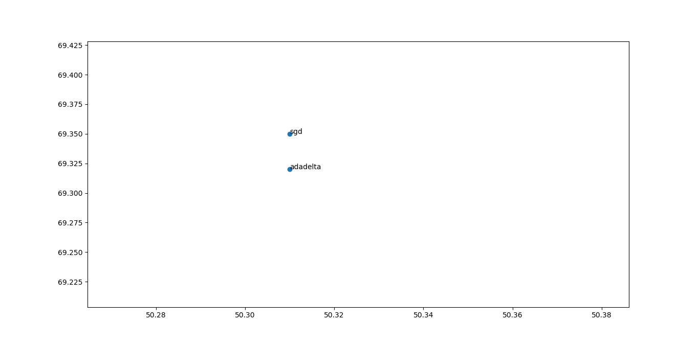
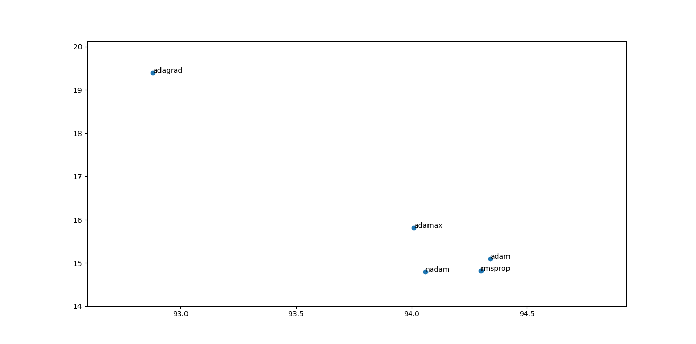
After tuning the different optimization algorithms , i have plotted the scatterplot to vizualise better for selection :
Scatterplot 1:
						x-axis : accuracy
						y-axis : Loss
Note : the above scatterplot is zoomed section of complete scatterplot.
Observation result:
By the above charts it is easy to sort out the reliable algorithms which are: adamax,adam,nadam,rmsprop amongs them the best suitable algorithm that i find useful is : adam ( because of higher accuracy with acceptable loss and rmsprop is better for RNN)
8.2 Loss
A loss function. This is the objective that the model will try to minimize. It can be the string identifier of an existing loss function (such as categorical_crossentropy or mse), or it can be an objective function.
The list of loss functions are :
1. Binary Crossentropy .
2. Mean Squared Error.
3. Mean Absolute Error.
4. Mean Squared Logrithmic error.
5. Squared Hing.
6. Hinge.
7. Poision.
8. Cosine Proximity.
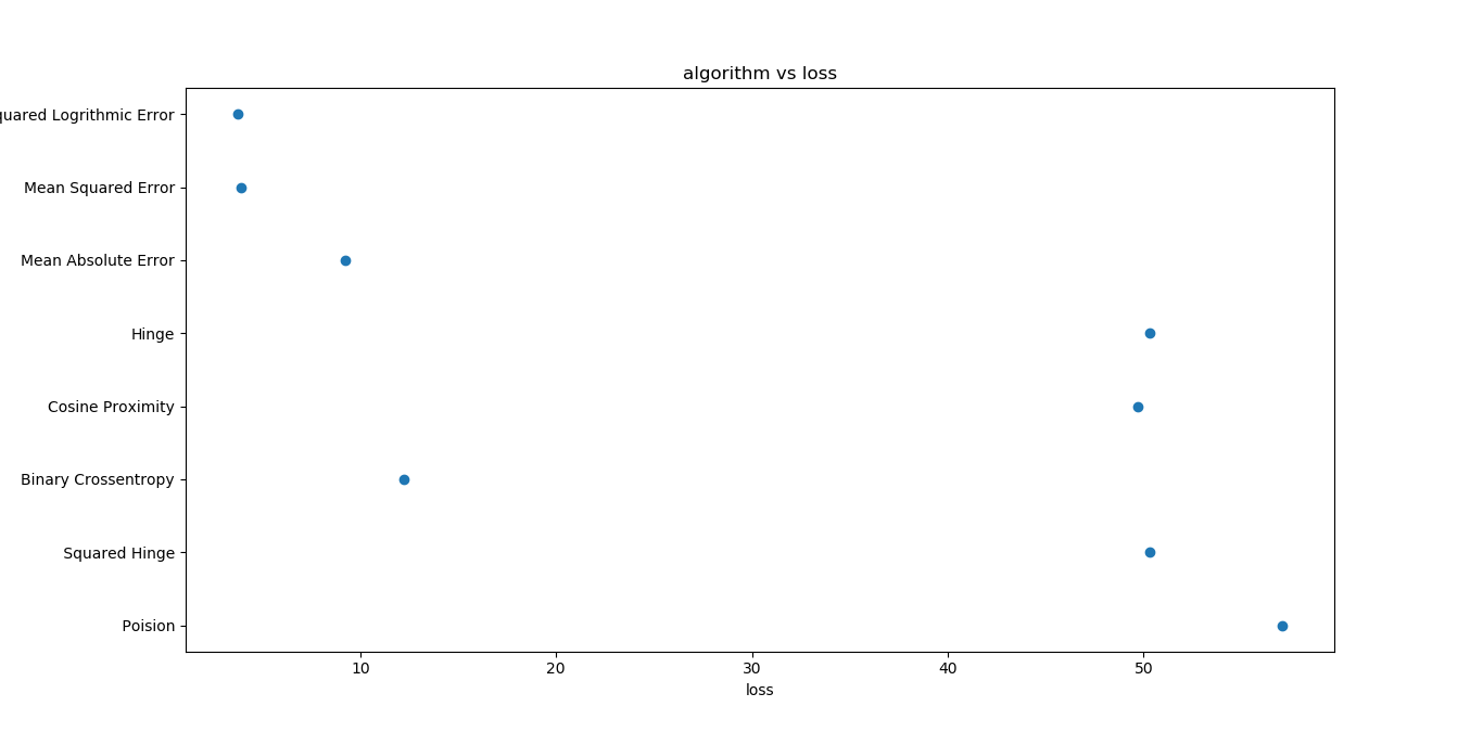
The below plot will be of help to vizualise and sort out the best function to minimize the losses.
Observation result:
From the above plot it is clear the Mean Squarred Error and Mean Squared Logrithmic Error both will be useful but depends of training accuracy.
8.3 Metric
A metric is a function that is used to judge the performance of your model. Metric functions are to be supplied in the metrics parameter when a model is compiled.
A list of metrics. For any classification problem you will want to set this to metrics=['accuracy']. A metric could be the string identifier of an existing metric or a custom metric function.
The list of metric function used to test are as follows :
1. Accuracy.
2. Binary Accuracy.
3. Categorical Accuracy.
4. Sparse Categorical Accuracy.
Keras defination to set metric function :
from keras import metrics

model.compile(loss='mean_squared_error',
              optimizer='sgd',
              metrics=[metrics.mae, metrics.categorical_accuracy])
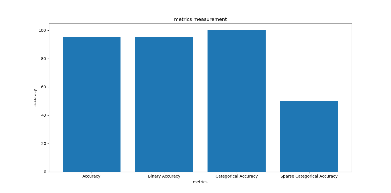
Bar chart will help in visualization better in this case :
Observation result:
It is clearly observable that categorical accuracy and binary accuracy are the most dominant one , hence giving the better results.
9 New Predictions
Now , we have a trained clasifier which can be used to predict the gender of audio files which is new (unseen).The trained classifier is saved in the folder called classifer.
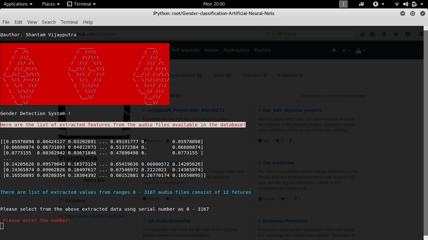
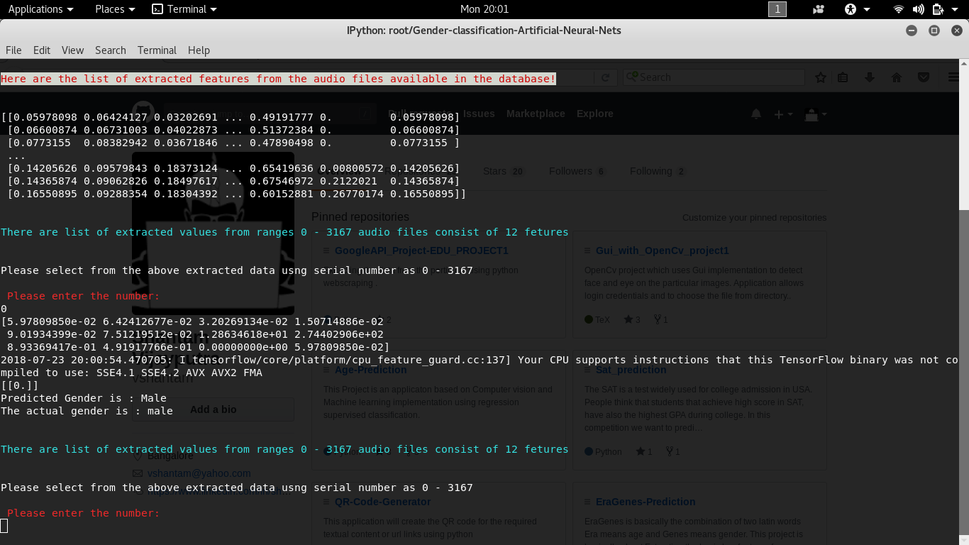
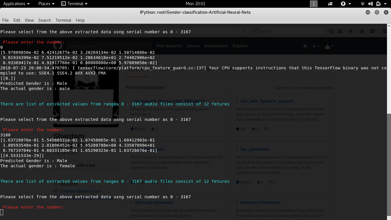
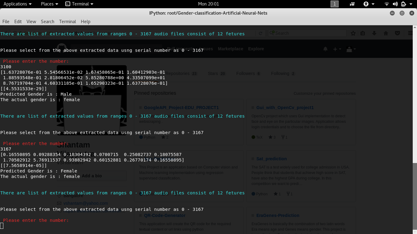
i am using a simple terminal based interface to use the pre trained classfier to predict the new values .
snapshots:
Main Interface
interface with correct prediction male
interface with false prediction
interface with correct prediction female
