- выбор оптимальных параметров катушек оповещателей для устаноки на внутритрубные дефектоскопы трубопроводов диаметром: 219 мм, 273 мм, 325 мм, 377 мм, 426 мм, 500 мм, 700 мм.

- проектирование и разработка библиотеки классов для моделирования катушек оповещателей в составе внутритрубных дефектоскопов
- тестирование методов классов на соответстие аналитическим методам решения
- эмпирическая проверка численных моделей (методов класса оповещателей)
- Метод определения электромагнитных свойств сердечника катушки
- разработка критериев эффективности: напряжённомсть магнитного поля, мощность активных потерь
- параметрических расчёт оповещателей и выбор оптимальных параметров.
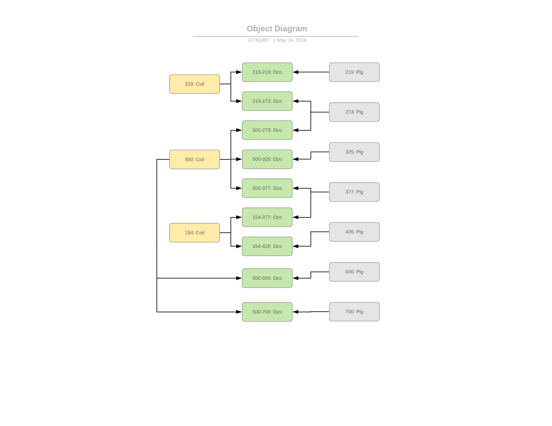
- design and development of a class library for modeling sounder coils as part of in-line flaw detectors
- testing of class methods for compliance with analytical methods of solution
- empirical verification of numerical models (sounder class methods)
- Method for determining the electromagnetic properties of a coil core
- building of performance criteria: magnetic field strength, active power loss
- parametric calculation and obtaining optimal parameters.


# coding=utf-8
import femm
from math import pi, sqrt, exp

# Диаметр провода выбирается из ряда diameterList
diameterList = [0.063, 0.071, 0.08, 0.09, 0.1, 0.112, 0.12, 0.125, 0.13, 0.14, 0.15, 0.16, 0.17, 0.18, 0.19, 0.2, 0.21,
                0.224, 0.236, 0.25, 0.265, 0.28, 0.3, 0.315, 0.335, 0.355, 0.38, 0.4, 0.425, 0.475, 0.45, 0.5, 0.53,
                0.56, 0.6, 0.63, 0.67, 0.69, 0.71, 0.75, 0.77, 0.8, 0.83, 0.85, 0.9, 0.93, 0.95, 1, 1.06, 1.12, 1.08,
                1.18, 1.25, 1.32, 1.4, 1.45, 1.5, 1.56, 1.6, 1.7, 1.8, 1.9, 2, 2.12, 2.24, 2.36, 2.44, 2.5]
class Wire(object):
'''
Создание объекта Провод
'''
version = '0.1' # class variable
def __init__(self, diameter):
'''
Initialize Wire Diameter in meters
'''
self.diameter = diameter
def area(self):
'''
Calculate wire Cross-sectional Area
'''
return pi * self.diameter ** 2 / 4class Coil(object):
def __init__(self, outerDiameter, innerDiameter, length, wireDiameter, fillFactor=57.3 / 100):
'''
Objects Inicialisation for Wire and Coil
'''
self.outerDiameter = outerDiameter
self.innerDiameter = innerDiameter
self.length = length
self.fillFactor = fillFactor
self.Wire = Wire(wireDiameter)
def area(self):
'''
Calculate coil cross-section area
'''
return (self.outerDiameter - self.innerDiameter) / 2 * self.length
def windingNomber(self):
'''
Calculate winding nomber in Coil
'''
return int(self.fillFactor * self.area() / self.Wire.area())
def wireLength(self):
'''
Calculate wire length in Coil
'''
return pi * self.windingNomber() * (self.outerDiameter + self.innerDiameter) / 2
def resistanceAnalitical(self):
""" Аналитический расчёт сопротивления катушки """
rho20 = 0.0172e-6 # (Ohm*mm^2)/m
return rho20 * self.wireLength() / self.Wire.area()class PIG(object):
def __init__(self, pipeOuterDiameter, pipeWall, modelName, voltage, freq=22, meshsize=1,
materials={'Сердечник': '1010 Steel', 'Дефектоскоп': '12H18N10T', 'Труба': '17G1S'}):
'''
Arguments:
-------------------
pipeOuterDiameter -- диаметр трубы в метрах
pipeWall -- толщина стенки трубы в метрах
Return:
-------------------
pointAt1mFromThePipe() -- координата X точки измерения поля на растоянии 1м от трубы
'''
self.pipeOuterDiameter = pipeOuterDiameter
self.pipeWall = pipeWall
self.modelName = modelName
self.voltage = voltage
self.freq = freq
self.meshsize = meshsize
self.materials = materials
def pointAt1mFromThePipe(self):
return self.pipeOuterDiameter / 2 + 1class OZO(object):
def __init__(self, Coil, PIG, results={}):
'''
здесь устанока атрибутов объекта и создание объектов Coil, PIG
'''
self.Coil = Coil
self.PIG = PIG
self.results = results
# Solving
def calculateModel(self, inputCurrentFund):
# =================== PreProcessing ===================
femm.openfemm(1)
femm.opendocument(self.PIG.modelName)
modelNameTemp = self.PIG.modelName.split('.')[0] + '_temp' + '.fem'
femm.mi_saveas(modelNameTemp)
# (0) Установка частоты тока
femm.mi_probdef(self.PIG.freq, 'millimeters', 'axi', 1e-8, 0, 30, 0)
# (1) Установка тока в обмотки
inputCurrentM = inputCurrentFund * sqrt(2)
femm.mi_setcurrent('New Circuit', inputCurrentM)
# (2) Изменеие диаметра провода
femm.mi_addmaterial(f'Wire d={self.Coil.Wire.diameter * 1000:.2f} mm',
1, 1, 0, 0, 58, 0, 0, 0, 3, 0, 0, 1, self.Coil.Wire.diameter * 1000)
# (3) Изменеие количества витков mi_setblockprop(’blockname’, automesh, meshsize,
# ’incircuit’, magdir, group, turns)
femm.mi_seteditmode('blocks')
femm.mi_selectgroup(1)
femm.mi_setblockprop(f'Wire d={self.Coil.Wire.diameter * 1000:.2f} mm', 0, 0.5,
'New Circuit', 0, 1, self.Coil.windingNomber())
# (4) Назначение материала для групп блоков FEM модели
femm.mi_zoom(0, -160, 150, 160)
groups = [2, 3, 4]
for index, group in enumerate(groups):
femm.mi_seteditmode('blocks')
femm.mi_clearselected()
femm.mi_selectgroup(group)
femm.mi_setblockprop(list(self.PIG.materials.values())[index], 0, self.PIG.meshsize, 0, 0, group, 0)
femm.mi_refreshview()
## =================== Расчёт ===================
femm.mi_analyze(1)
femm.closefemm()
print(f'Предварительная модель "{modelNameTemp}" готова (f = {self.PIG.freq:.1f}Hz)')
return modelNameTemp
def CalculateModel2Steps(self, plotPie=0):
# ============== <1-й прогон> ==============
print(
f'''<<< 1st step ({self.Coil.Wire.diameter * 1000:.3f} mm) x {self.Coil.windingNomber()} витков, Сопротивление обмотки аналитически = {self.Coil.resistanceAnalitical():.3} Ом>>>
Материалы = {self.PIG.materials}''')
# Solve()
tempModelName = self.calculateModel(inputCurrentFund=self.PIG.voltage / self.Coil.resistanceAnalitical())
# Post Processing
# tempModelName = "OZO-500_Full_temp.fem"
(coilFieldIntensityAt1m, coilInductatce, activeImpedanceNames, activeImpedance, activePowerLoss,
coilVoltageDrop) = self.getImpedance(modelNameTemp=tempModelName)
# ============== <2-й прогон> ==============
# Задание режима по вычисленому импедансу
fullImpedance = abs(sum(activeImpedance) + 1j * 2 * pi * self.PIG.freq * coilInductatce)
Im = self.PIG.voltage / fullImpedance
Ifund = Im / sqrt(2)
nominalCurrent = Ifund
print(
f'<<< 2nd step ({self.Coil.Wire.diameter * 1000:.3f} mm) x {self.Coil.windingNomber()} витков, nominalCurrent = {nominalCurrent:.3f} А >>>')
# Solve()
tempModelName = self.calculateModel(nominalCurrent)
# Post Processing
(coilFieldIntensityAt1m, coilInductatce, activeImpedanceNames, activeImpedance, activePowerLoss,
coilVoltageDrop) = self.getImpedance(modelNameTemp=tempModelName)
if plotPie == 1:
self.PlotLosesPie(activeImpedanceNames, activePowerLoss)
return [coilFieldIntensityAt1m, coilInductatce, activeImpedanceNames, activeImpedance, activePowerLoss,
coilVoltageDrop, nominalCurrent]
# PostProcessing
def calculateInductance(self, group):
'''вычисление индуктивности через A · J
'''
from math import pi, sqrt
inputCurrentM = femm.mo_getcircuitproperties('New Circuit')[0]
currentFund = inputCurrentM / sqrt(2)
femm.mo_groupselectblock(group)
inductance = femm.mo_blockintegral(0) / inputCurrentM ** 2 # A·J
femm.mo_clearblock()
return inductance.real
def calculateActiveImpedance(self, group):
'''
Функция возращает значение активного импеданса (R) и мощности потерь (TotalLoses)
R, TotalLosses = calculateActiveImpedance(currentFund)
'''
from math import pi, sqrt
inputCurrentM = femm.mo_getcircuitproperties('New Circuit')[0]
currentFund = inputCurrentM / sqrt(2)
femm.mo_groupselectblock(group)
TotalLosses = femm.mo_blockintegral(6) # Total losses
femm.mo_clearblock()
return abs(TotalLosses / currentFund ** 2), abs(TotalLosses)
def getImpedance(self, modelNameTemp):
# from math import pi, sqrt
femm.openfemm(1)
femm.opendocument(modelNameTemp)
# Get CoilCerrentM from model
femm.mi_loadsolution()
# Расчёт напряжённости магнитного поля на расстоянии 1 м от трубы
# PipeDiameter = float(modelNameTemp.split('-')[1].split('_')[0])
(Hr, Hz) = femm.mo_getpointvalues(self.PIG.pointAt1mFromThePipe() * 1000, 0)[5:7]
coilFieldIntensityAt1m = abs(Hz) # раньше было abs(Hr + Hz)
# Получение амплитуды магнитного поля в катушке для последующего расчёта компонет импеданса
inputCurrentM = femm.mo_getcircuitproperties('New Circuit')[0]
currentFund = inputCurrentM / sqrt(2)
activeImpedanceNames = ['Обмотка', 'Сердечник', 'Дефектоскоп', 'Труба']
(activeImpedance, activePowerLoss) = ([], [])
for group in range(4):
# print('group_{}. '.format(group))
(activeImpedance_, activePowerLoss_) = self.calculateActiveImpedance(group + 1) # calculateActiveImpedance
activeImpedance.append(activeImpedance_)
activePowerLoss.append(activePowerLoss_)
# print('{}: activeImpedance = {:.3f} Ohm, activePowerLoss = {:.3f} W'.format(activeImpedanceNames[group],
# activeImpedance_,
# activePowerLoss_))
if group == 0:
coilInductatce = self.calculateInductance(group + 1)
# print('coilInductatce = {:.1f} mH'.format(coilInductatce * 1000))
coilVoltageDrop = femm.mo_getcircuitproperties('New Circuit')[1]
# print('voltage Drop = {}'.format(abs(coilVoltageDrop)))
print(f'''=======================================================================
Напряжённость поля на расстоянии 1 м от трубы = {coilFieldIntensityAt1m:.2e} А/м''')
# print(f'''Индуктивность = {coilInductatce*1000:c4} мГн, Суммарный активный импеданс = {sum(activeImpedance):.3} Ом
# Суммарные активные потери = {sum(activePowerLoss):.3} Вт
# Падение напряжения на катушке = {abs(coilVoltageDrop):.3} В (ампл) {abs(coilVoltageDrop)/sqrt(2):.3} В (fund)
# ''')
femm.closefemm()
return coilFieldIntensityAt1m, coilInductatce, \
activeImpedanceNames, activeImpedance, activePowerLoss, coilVoltageDrop
def PlotLosesPie(self, labels, loses):
'''
Arguments:
-------------------
labels -- if !=0 prints names of Coils, Pigs and Ozos to be initialised
loses
Return:
-------------------
'''
import matplotlib.pyplot as plt
# Pie chart, where the slices will be ordered and plotted counter-clockwise:
data = [abs(loses) for loses in loses]
OveralLoses = abs(sum(data))
sizes = [val / OveralLoses for val in data]
explode = (0, 0.1, 0, 0) # only "explode" the 2nd slice (i.e. 'Hogs')
fig1, ax1 = plt.subplots() # figsize=(12, 9)
ax1.pie(sizes, explode=explode, labels=labels, autopct='%1.1f%%', shadow=True, startangle=90)
ax1.axis('equal') # Equal aspect ratio ensures that pie is drawn as a circle.
ax1.set_title("Суммарные активные потери = {:.3f} Вт".format(OveralLoses))
plt.show()
