`caribou_hi`

A Bayesian Model of the Diffuse Neutral Interstellar Medium

caribou_hi is a Bayesian model of the diffuse neutral interstellar medium written in the bayes_spec spectral line modeling framework, which enables inference from observations of neutral hydrogen (HI) 21-cm emission and absorption spectra.

Read below to get started, and check out the tutorials and guides here: https://caribou-hi.readthedocs.io.

Installation
- Basic Installation
- Development Installation
Notes on Physics & Radiative Transfer
Models
Syntax & Examples
Issues and Contributing
License and Copyright

Installation

Basic Installation

Install with pip in a conda virtual environment:

conda create --name caribou_hi -c conda-forge pymc nutpie pip
conda activate caribou_hi
pip install caribou_hi

Development Installation

Alternatively, download and unpack the latest release, or fork the repository and contribute to the development of caribou_hi!

Install in a conda virtual environment:

cd /path/to/caribou_hi
conda env create -f environment.yml
conda activate caribou_hi-dev
pip install -e .

Notes on Physics & Radiative Transfer

All models in caribou_hi apply the same physics and equations of radiative transfer.

The 21-cm excitation temperature (also called the spin temperature) is derived from the gas kinetic temperature, gas density, and Lyα photon density following Kim et al. (2014) equation 4.

Clouds are assumed to be homogenous and isothermal. The ratio of the column density to the volume density, both free parameters, thus determines the path length through the cloud. The non-thermal line broadening assumes a Larson law relationship.

The optical depth and radiative transfer prescriptions follow that of Marchal et al. (2019). By default, the clouds are ordered from nearest to farthest, so optical depth effects (i.e., self-absorption) may be present.

Notably, since these are forward models, we do not make assumptions regarding the optical depth. These effects are predicted by the model. There is one exception: the ordered argument, described below.

Models

The models provided by caribou_hi are implemented in the bayes_spec framework. bayes_spec assumes that the source of spectral line emission can be decomposed into a series of "clouds", each of which is defined by a set of model parameters. Here we define the models available in caribou_hi.

`EmissionModel`

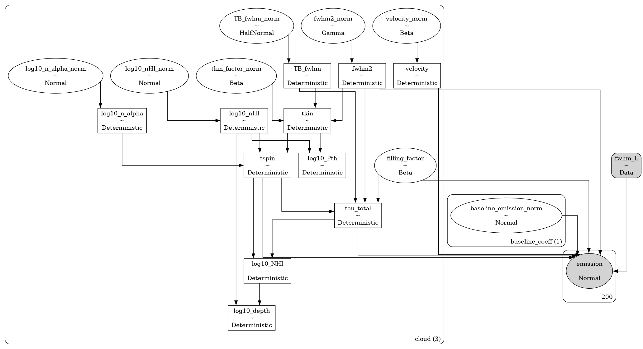
EmissionModel is a model that predicts 21-cm emission brightness temperature spectra. The SpecData key for this model must be emission. The following diagram demonstrates the relationship between the free parameters (empty ellipses), deterministic quantities (rectangles), model predictions (filled ellipses), and observations (filled, round rectangles). Many of the parameters are internally normalized (and thus have names like _norm). The subsequent tables describe the model parameters in more detail.

Cloud Parameter `variable`	Parameter	Units	Prior, where ($p_0, p_1, \dots$) = `prior_{variable}`	Default `prior_{variable}`
`log10_NHI`	log10 HI column density	`cm-2`	$\log_{10}N_{\rm HI} \sim {\rm Normal}(\mu=p_0, \sigma=p_1)$	`[20.0, 1.0]`
`log10_nHI`	log10 HI density	`cm-3`	$\log_{10}n \sim {\rm Normal}(\mu=p_0, \sigma=p_1)$	`[0.0, 1.0]`
`log10_tkin`	log10 kinetic temperature	`K`	$\log_{10}T_K \sim {\rm Normal}(\mu=p_0, \sigma=p_1)$	`[3.0, 1.0]`
`log10_n_alpha`	log10 Lyα photon density	`cm-3`	$\log_{10}n_\alpha \sim {\rm Normal}(\mu=p_0, \sigma=p_1)$	`[-6.0, 1.0]`
`log10_larson_linewidth`	Non-thermal broadening FWHM at 1 pc	`km s-1`	$\log_{10}\Delta V_{\rm 1 pc} \sim {\rm Normal}(\mu=p_0, \sigma=p_1)$	`[0.2, 0.1]`
`larson_power`	Nonthermal size-linewidth power law index	unitless	$\alpha \sim {\rm Normal}(\mu=p_0, \sigma=p_1)$	`[0.4, 0.1]`
`velocity`	Velocity (same reference frame as data)	`km s-1`	$V \sim {\rm Normal}(\mu=p_0, \sigma=p_1)$	`[0.0, 10.0]`

Hyper Parameter `variable`	Parameter	Units	Prior, where ($p_0, p_1, \dots$) = `prior_{variable}`	Default `prior_{variable}`
`rms_emission`	Emission spectrum rms noise	`K`	${\rm rms}_{T} \sim {\rm HalfNormal}(\sigma=p)$	`1.0`

`AbsorptionModel`

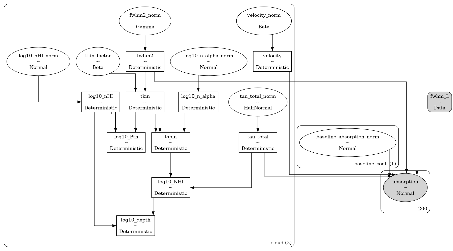
AbsorptionModel is otherwise identical to EmissionModel, except it predicts 21-cm optical depth spectra. The SpecData key for this model must be absorption. The following diagram demonstrates the model, and the subsequent table describe the additional model parameters.

Cloud Parameter `variable`	Parameter	Units	Prior, where ($p_0, p_1, \dots$) = `prior_{variable}`	Default `prior_{variable}`
`log10_NHI`	log10 HI column density	`cm-2`	$\log_{10}N_{\rm HI} \sim {\rm Normal}(\mu=p_0, \sigma=p_1)$	`[20.0, 1.0]`
`log10_nHI`	log10 HI density	`cm-3`	$\log_{10}n \sim {\rm Normal}(\mu=p_0, \sigma=p_1)$	`[0.0, 1.0]`
`log10_tkin`	log10 kinetic temperature	`K`	$\log_{10}T_K \sim {\rm Normal}(\mu=p_0, \sigma=p_1)$	`[3.0, 1.0]`
`log10_n_alpha`	log10 Lyα photon density	`cm-3`	$\log_{10}n_\alpha \sim {\rm Normal}(\mu=p_0, \sigma=p_1)$	`[-6.0, 1.0]`
`log10_larson_linewidth`	Non-thermal broadening FWHM at 1 pc	`km s-1`	$\log_{10}\Delta V_{\rm 1 pc} \sim {\rm Normal}(\mu=p_0, \sigma=p_1)$	`[0.2, 0.1]`
`larson_power`	Nonthermal size-linewidth power law index	unitless	$\alpha \sim {\rm Normal}(\mu=p_0, \sigma=p_1)$	`[0.4, 0.1]`
`velocity`	Velocity (same reference frame as data)	`km s-1`	$V \sim {\rm Normal}(\mu=p_0, \sigma=p_1)$	`[0.0, 10.0]`

Hyper Parameter `variable`	Parameter	Units	Prior, where ($p_0, p_1, \dots$) = `prior_{variable}`	Default `prior_{variable}`
`rms_absorption`	Optical depth spectrum rms noise	`K`	${\rm rms}_{\tau} \sim {\rm HalfNormal}(\sigma=p)$	`0.01`

`EmissionAbsorptionModel`

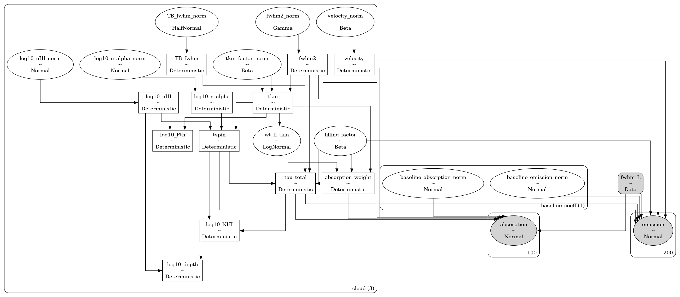
EmissionAbsorptionModel predicts both 21-cm emission (brightness temperature) and optical depth spectra assuming that both observations trace the same gas. The SpecData keys must be emission and absorption. The following diagram demonstrates the model, and the subsequent table describe the additional model parameters.

Cloud Parameter `variable`	Parameter	Units	Prior, where ($p_0, p_1, \dots$) = `prior_{variable}`	Default `prior_{variable}`
`log10_NHI`	log10 HI column density	`cm-2`	$\log_{10}N_{\rm HI} \sim {\rm Normal}(\mu=p_0, \sigma=p_1)$	`[20.0, 1.0]`
`log10_nHI`	log10 HI density	`cm-3`	$\log_{10}n \sim {\rm Normal}(\mu=p_0, \sigma=p_1)$	`[0.0, 1.0]`
`log10_tkin`	log10 kinetic temperature	`K`	$\log_{10}T_K \sim {\rm Normal}(\mu=p_0, \sigma=p_1)$	`[3.0, 1.0]`
`log10_n_alpha`	log10 Lyα photon density	`cm-3`	$\log_{10}n_\alpha \sim {\rm Normal}(\mu=p_0, \sigma=p_1)$	`[-6.0, 1.0]`
`log10_larson_linewidth`	Non-thermal broadening FWHM at 1 pc	`km s-1`	$\log_{10}\Delta V_{\rm 1 pc} \sim {\rm Normal}(\mu=p_0, \sigma=p_1)$	`[0.2, 0.1]`
`larson_power`	Nonthermal size-linewidth power law index	unitless	$\alpha \sim {\rm Normal}(\mu=p_0, \sigma=p_1)$	`[0.4, 0.1]`
`velocity`	Velocity (same reference frame as data)	`km s-1`	$V \sim {\rm Normal}(\mu=p_0, \sigma=p_1)$	`[0.0, 10.0]`

Hyper Parameter `variable`	Parameter	Units	Prior, where ($p_0, p_1, \dots$) = `prior_{variable}`	Default `prior_{variable}`
`rms_emission`	Emission spectrum rms noise	`K`	${\rm rms}_{T} \sim {\rm HalfNormal}(\sigma=p)$	`1.0`
`rms_absorption`	Optical depth spectrum rms noise	`K`	${\rm rms}_{\tau} \sim {\rm HalfNormal}(\sigma=p)$	`0.01`

`EmissionAbsorptionFFModel`

Finally, EmissionAbsorptionFFModel is like EmissionAbsorptionModel, except it allows for the possibility of beam dilution in the emission spectrum. That is, the expected brightness temperature contribution from a cloud is modified by a parameter, filling_factor, which takes values between zero and one.

Cloud Parameter `variable`	Parameter	Units	Prior, where ($p_0, p_1, \dots$) = `prior_{variable}`	Default `prior_{variable}`
`filling_factor`	Filling Factor	``	$f \sim 1.0 - {\rm Beta}(\alpha=1.0, \beta=2.0)$	``

`ordered`

An additional parameter to set_priors for these models is ordered. By default, this parameter is False, in which case the order of the clouds is from nearest to farthest. Sampling from these models can be challenging due to the labeling degeneracy: if the order of clouds does not matter (i.e., the emission is optically thin), then each Markov chain could decide on a different, equally-valid order of clouds.

If we assume that the emission is optically thin, then we can set ordered=True, in which case the order of clouds is restricted to be increasing with velocity. This assumption can drastically improve sampling efficiency. When ordered=True, the velocity prior is defined differently:

Cloud Parameter `variable`	Parameter	Units	Prior, where ($p_0, p_1, \dots$) = `prior_{variable}`	Default `prior_{variable}`
`velocity`	Velocity	`km s-1`	$V_i \sim p_0 + \sum_0^{i-1} V_i + {\rm Gamma}(\alpha=2, \beta=1.0/p_1)$	`[0.0, 1.0]`

Syntax & Examples

See the various tutorial notebooks under docs/source/notebooks. Tutorials and the full API are available here: https://caribou-hi.readthedocs.io.

Issues and Contributing

Anyone is welcome to submit issues or contribute to the development of this software via Github.

License and Copyright

GNU General Public License v3 (GNU GPLv3)

This program is free software: you can redistribute it and/or modify it under the terms of the GNU General Public License as published by the Free Software Foundation, either version 3 of the License, or (at your option) any later version.

This program is distributed in the hope that it will be useful, but WITHOUT ANY WARRANTY; without even the implied warranty of MERCHANTABILITY or FITNESS FOR A PARTICULAR PURPOSE. See the GNU General Public License for more details.

You should have received a copy of the GNU General Public License along with this program. If not, see http://www.gnu.org/licenses/.

tvwenger / caribou_hi