RStudio Connect Usage Data

This repository illustrates several examples for getting started with the RStudio Connect usage data. The examples:

The examples are generated using the RStudio Connect Server API. The API and data collection are both available as of RStudio Connect 1.7.0. The API contains data to help answer questions like:

What content is most visited?
Who is visiting my content?
What reports are most common?
Has viewership increased over time?
Did my CEO actually visit this app?

A data science team’s time is precious, this data will help you focus and justify your efforts.

Basic example

The following code should work as-is if copied into your R session. NOTE that it uses the connectapi package, which can be installed from GitHub with remotes::install_github("rstudio/connectapi"). You just need to replace the server name, and have your API key ready.

## ACTION REQUIRED: Change the server URL below to your server's URL
Sys.setenv("CONNECT_SERVER"  = "https://connect.example.com/rsc") 
## ACTION REQUIRED: Make sure to have your API key ready
Sys.setenv("CONNECT_API_KEY" = rstudioapi::askForPassword("Enter Connect Token:"))

This will use the get_usage_shiny() function to pull the latest activity of the Shiny apps you are allowed to see within your server.

library(ggplot2)
library(dplyr)
library(connectapi)

client <- connect()

# Get and clean the Shiny usage data
shiny_rsc <- get_usage_shiny(
  client,
  from = lubridate::today() - lubridate::ddays(7), 
  limit = Inf
  ) %>%
  filter(!is.na(ended)) %>%
  mutate(session_duration = ended - started)

glimpse(shiny_rsc)

## Rows: 336
## Columns: 6
## $ content_guid     <chr> "dad2ac84-2450-4275-b26e-8e0d9d741100", "6f69884b-562…
## $ user_guid        <chr> NA, NA, NA, NA, NA, NA, NA, "7defcf1b-69f6-4bc5-8b52-…
## $ started          <dttm> 2022-02-23 01:54:12, 2022-02-23 03:17:46, 2022-02-23…
## $ ended            <dttm> 2022-02-23 01:54:45, 2022-02-23 03:19:25, 2022-02-23…
## $ data_version     <int> 1, 1, 1, 1, 1, 1, 1, 1, 1, 1, 1, 1, 1, 1, 1, 1, 1, 1,…
## $ session_duration <drtn> 33 secs, 99 secs, 3685 secs, 61 secs, 59 secs, 51 se…

The identifiers used for the content in RStudio Connect are GUIDs. We can retrieve content names using the API. The API handles only one GUID at a time, so purrr’s map_dfr() is used to iterate through all of the unique GUIDs in order to get every Shiny app’s title.

# Get the title of each Shiny app
shiny_rsc_titles <- shiny_rsc %>%
  count(content_guid) %>% 
  pull(content_guid) %>%
  purrr::map_dfr(
    ~tibble(content_guid = .x, content_name = content_title(client, .x))
    )

glimpse(shiny_rsc_titles)

## Rows: 40
## Columns: 2
## $ content_guid <chr> "0287f7d9-4d55-4813-8852-680f54beaad1", "06484fbb-f686-42…
## $ content_name <chr> "Example Palmer Penguins Shiny Dashboard", "Classroom Stu…

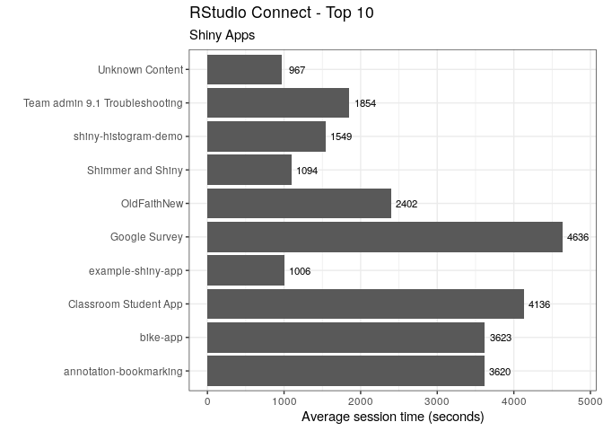
The new shiny_rsc_titles table, and the shiny_rsc can be joined to return the “user readable” title. Using standard dplyr and ggplot2 functions, we can now determine things such as the top 10 apps based on how long their average sessions are.

# Calculate the average session duration and sort
app_sessions <- shiny_rsc %>%
  inner_join(shiny_rsc_titles, by = "content_guid") %>%
  group_by(content_name) %>%
  summarise(avg_session = mean(session_duration)) %>%
  ungroup() %>%
  arrange(desc(avg_session)) %>%
  head(10)
  
# Plot the top 10 used content
app_sessions %>%
  ggplot(aes(content_name, avg_session)) +
  geom_col() +
  scale_y_continuous() +
  geom_text(aes(y = (avg_session + 200), label = round(avg_session)), size = 3) +
  coord_flip() +
  theme_bw() +
  labs(
    title = "RStudio Connect - Top 10", 
    subtitle = "Shiny Apps", 
    x = "", 
    y = "Average session time (seconds)"
    )

Learn more about programmatic deployments, calling the server API, and custom emails here.

tburnley / connect-usage

RStudio Connect Usage Data

Basic example

About

Languages