sysu-ccy / kozaipy

Secular equations of motion for the evolution of triple systems with tidal friction

KOZAIPY - Secular equations of motion for the evolution of triple systems with tidal friction

Welcome to KozaiPy!

Overview

KozaiPy is a Python package for the integration of the secular equations of motion of few-body hierarchical systems.

Installation

You need to have git installed. In addition, you need the NumPy and SciPy Python packages.

git clone https://github.com/djmunoz/kozaipy.git

cd kozaipy

sudo python setup.py install

That is all!

Examples

1. Orbital flips

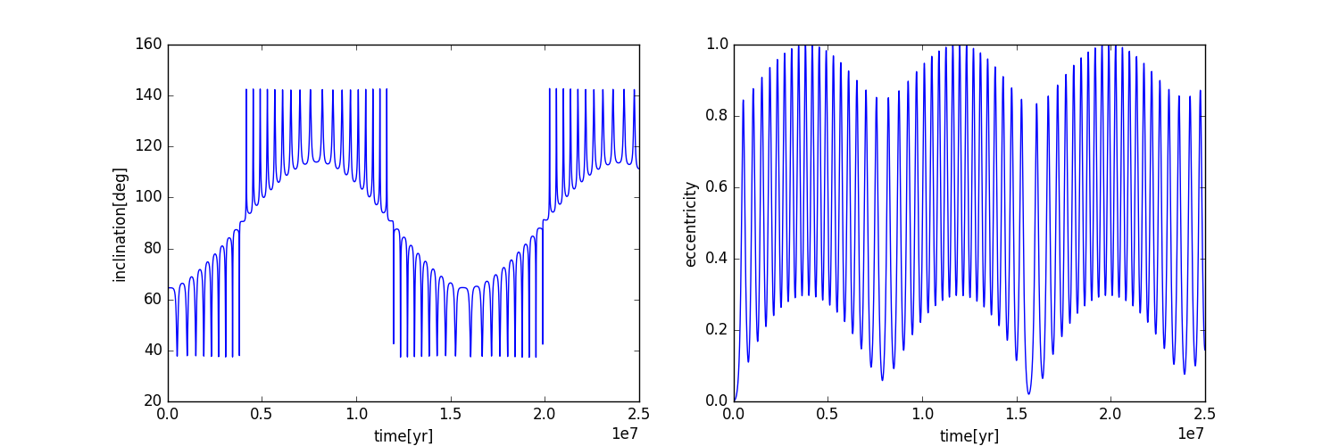
   To run a secular triple (e.g. Fig.3 of Naoz et al 2013). First setup the triple

as:

import kozaipy as kp
import numpy as np

trip = kp.Triple(m0=1.0,m1=0.001,m2=0.04,a1=6.0,a2=100.0,e1=0.001,e2=0.6,\
       I=65.0 * np.pi/180.0, g1=45.0 * np.pi/180.0,g2=0)

And then evolve the system for 2.5e7 years

sol = trip.integrate(timemin=0.0,timemax=2.5e7*365.25,Nevals=30000,octupole_potential=True)

The equations of motion are in the 'orbital vector form' (e.g., Eggleton, Kiseleva & Hut 1998; Fabrycky & Tremaine, 2007; Tremaine & Yavetz, 2014) and so is the solution output. If you want to analyze the orbital elements, first do:

sol.to_elements()

To plot the inclination and eccentricity of the inner orbit, simply do

import matplotlib.pyplot as plt

time = sol.vectordata.time
incl1= sol.elementdata.I1
ecc1 = sol.elementdata.e1

fig = plt.figure(figsize=(15,5))
ax = plt.subplot(121)
ax.set_xlabel("time[yr]")
ax.set_ylabel("inclination[deg]")
ax.plot(time/365.25,incl1)


ax = plt.subplot(122)
ax.set_xlabel("time[yr]")
ax.set_ylabel("eccentricity")
ax.plot(time/365.25,ecc1)
plt.show()

You should get something like this:

You can save the data into a text file by doing

sol.save_to_file("test.txt",Nlines=None)

where 'Nlines' allows you to set a lower number of lines than the original solution.

2. High-e migration: HD80606b

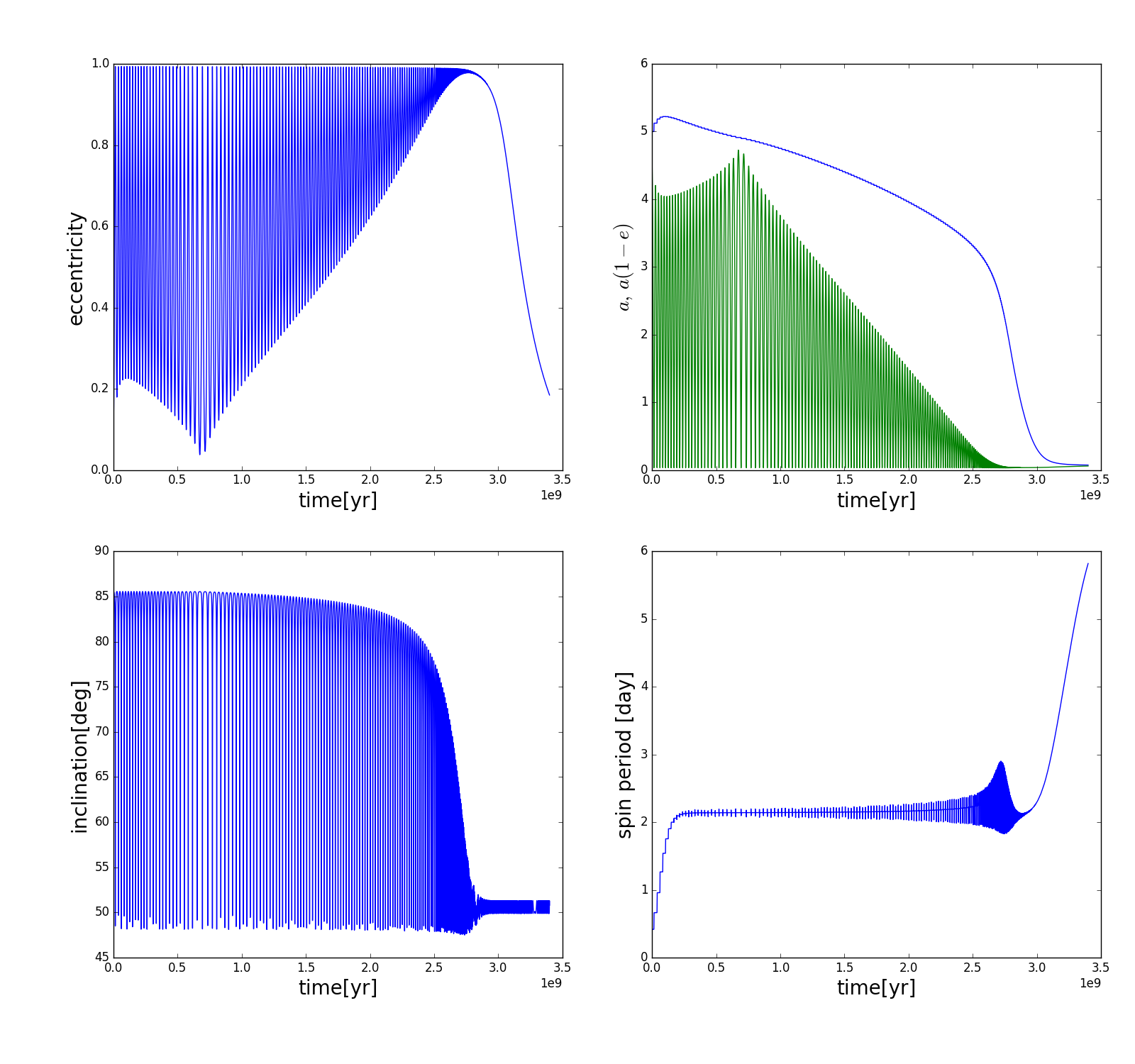
Following the model of Wu & Murray (2003), we can setup a triple that resultins in a configuration similar to that of HD80606b

trip = kp.Triple(m0=1.1,m1=0.007443,m2=1.1,a1=5.0,a2=1000.0,e1=0.1,e2=0.5,I=85.6 * np.pi/180.0, \
       g1=45.0 * np.pi/180.0,g2=0.0,\
       type0='star',type1='planet',\
       spinorbit_align0=False,\
       spinorbit_align1=True,\
       spin_rate0 = 2 * np.pi/20, spin_rate1 = 2 * np.pi/0.417,
       R0=kp.constants.Rsun,R1=kp.constants.Rsun/10,
       k2_0 = 0.014, k2_1=0.25, tv0=2.0e4, tv1=0.365242,rg_0=0.08,rg_1=0.25)

We integrate this sytem in time including tidal friction. For that, we turn on the two options 'short_range_forces_conservative' and 'short_range_forces_dissipative'

sol = trip.integrate(timemin=0.0,timemax=3.4e9*365.25,Nevals=12000,\
       octupole_potential=False,\
       short_range_forces_conservative=True, \
       short_range_forces_dissipative=True)

Note that we also turn off the octupole potential for now, for easier comparison with Wu & Murray (2003) and Fabrycky & Tremaine (2007):

The dissipative forces make the system of ODEs stiff, and turning them on can slow down this integration from a few seconds to up to an hour. I am still working on this, but a speed up will probably require a purpose-specific ODE solver rather than using the ODEPACK routines implemented in scipy.