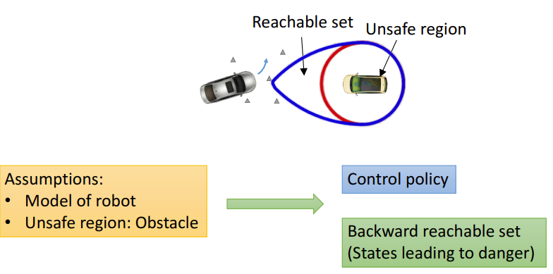
Optimized Dynamic Programming-Based Algorithms Solver (OptimizedDP)

The repo contains implementation of dynamic programming based algorithms in optimal control. Specifically, the solver supports 3 main classes of algorithms: level set based algorithm for solving Hamilton-Jacobi-Issac (HJI) partial differential equation (PDE) arising in reachability analysis and differential games [1], time-to-reach (TTR) computations of dynamical systems in reachability analysis [2], and value-iterations algorithm for solving continuous state-space action-space Markov Decision Process (MDP). All these algorithms share the property of being implemented on a multidimensional grid and hence, their computational complexities increase exponentially as a function of dimension. For all the aforementioned algorithms, our toolbox allows computation up to 6 dimensions, which we think is the limit of dynammic programming on most modern personal computers.

In comparison with previous works, our toolbox strives to be both efficient in implementation while being user-friendly. This is reflected in our choice of having Python as a language for initializing problems and having python-like HeteroCL [3] language for the core algorithms implementation and dynamical systems specification. Our implementation is 7-32x faster than the Level Set Toolbox and HelperOC and 2-3x faster than BEACLS implementation in C++. Please find more details about using the repo for solving your problems in this page, and should you have any questions/problems/requests please direct the messages to Minh Bui at buiminhb@sfu.ca

Quickstart (Ubuntu 18 & 20)

Please install the following:

Install Anaconda (https://docs.anaconda.com/anaconda/install/linux/)
Install heteroCL (http://heterocl.csl.cornell.edu/doc/installation.html):

Create new conda environment: conda create --name hcl-env

Activate new conda environment: conda activate hcl-env

Install pre-built heterocl: conda install -c cornell-zhang heterocl -c conda-forge

Note: You might also need to install module "future" if encounter an error, with this command pip3 install future.
Potential Python modules to install if you run into errors:

pip3 install future plotly==4.5.0
Run the example code from optimized_dp root directory: python3 examples.py
Note: If you're on Ubuntu 20.04, you may have encounter an error regarding libtinfo5. To fix, please just run this command sudo apt-install libtinfo5

Solving the Hamilton-Jacobi-Issac (HJI) PDE

We provide a running example of solving HJI PDE in the file examples.py:

g = Grid(np.array([-4.0, -4.0, -math.pi]), np.array([4.0, 4.0, math.pi]), 3, np.array([40, 40, 40]), [2])

# A sphere shape (no dimension passed in) 
Initial_value_f = CylinderShape(g, [], np.zeros(3), 1)

# Look-back length and time step
lookback_length = 2.0
t_step = 0.05

small_number = 1e-5
tau = np.arange(start=0, stop=lookback_length + small_number, step=t_step)

# User-defined system dynamcics
my_car = DubinsCapture()

po2 = PlotOptions(do_plot=False, plot_type="3d_plot", plotDims=[0,1,2],
                  slicesCut=[])
                  
# Computing Backward Reachable-Tube (BRT)
compMethods = { "PrevSetsMode": "minVWithV0"}
result = HJSolver(my_car, g, Initial_value_f, tau, compMethods, po2, saveAllTimeSteps=True )

To run the example, execute the command python3 examples.py
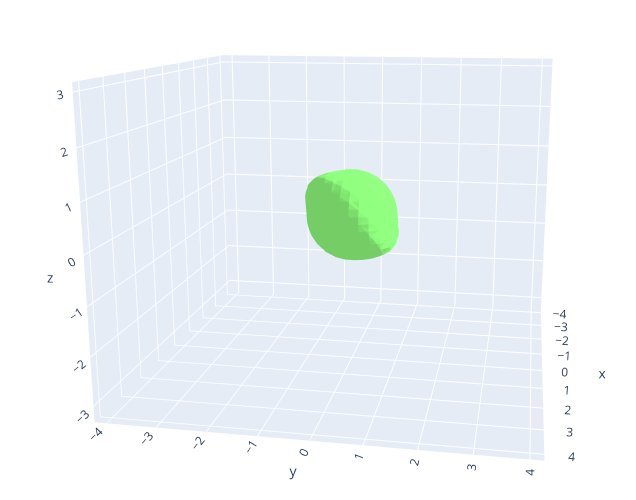
If the parameter do_plot is set to True when initializing PlotOptions, there will be a 3D green colored sub-zero level set popping up in your default browser like below.

Notes: For 6 dimensions, recommended grid size is 20-30 each dimension on system with 32Gbs of DRAM.
Create a class file in folder dynamics/ to specify your own system dynamics. Remember to import the class in your running example.

Time-to-Reach computation

We have provided an example in TTR_example.py:

# -------------------------------- ONE-SHOT TTR COMPUTATION ---------------------------------- #
g = Grid(minBounds=np.array([-3.0, -1.0, -math.pi]), maxBounds=np.array([3.0, 4.0, math.pi]),
         dims=3, pts_each_dim=np.array([50, 50, 50]), periodicDims=[2])
# Car is trying to reach the target
my_car = DubinsCar(uMode="min")

# Initialize target set as a cylinder
targetSet = CylinderShape(g, [2], np.array([0.0, 1.0, 0.0]), 0.70)
po = PlotOptions( "3d_plot", plotDims=[0,1,2], slicesCut=[],
                  min_isosurface=lookback_length, max_isosurface=lookback_length)

# Convergence threshold
epsilon = 0.001
V_0 = TTRSolver(my_car, g, targetSet, epsilon, po)

To run the example : python3 TTR_example.py

Current code structure

solver.py: Containing python APIs to interact with the numerical solver
dynamics/ : User's dynamical system specification
Shapes/ShapesFunctions.py : Add-in functions for initializing different shapes/intial value functions
computeGraphs/CustomGraphFunctions.py: Ready-to-user HeteroCL style utility functions

Related Projects

MATLAB

C++

BEACLS

Python/JAX

hj_reachability

References

[1] "Hamilton–Jacobi Reachability: Some Recent Theoretical Advances and Applications in Unmanned Airspace Management" by Mo Chen and Claire J. Tomlin in Annual Review of Control, Robotics, and Autonomous Systems 2018 1:1, 333-358 pdf

[2] "One-Shot Computation of Reachable Sets for Differential Games" by Insoon Yang pdf

[3] "HeteroCL: A Multi-Paradigm Programming Infrastructure for Software-Defined Reconfigurable Computing" by Yi-Hsiang Lai pdf

sudo-michael / optimized_dp