Research Paper: An Image is Worth 16x16 Words: Transformers for Image Recognition at Scale
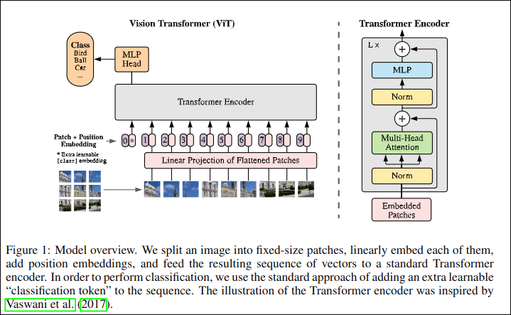
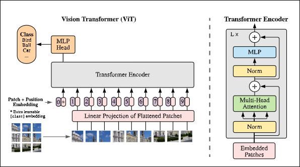
- figure 1: visual overview of the architecture
- four equations: math equations which define the function of each layer/block
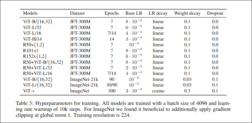
- table 1/3: different hyperparameters for the architecture/training.
- text
- embedding - learnable representation (start with random numbers and improve them overtime)
- mlp = multilevel perceptron
Equaion1:
- embedding - learnable representation (start with random numbers and improve them overtime)
- path embeddings - patches of original image - pink
- position embeddings - to retain positional information - purple
- class token embedding - to perform classification (*/pink)
x_input = [learnable_class_token, image_patch_embeddings_1, image_patch_embeddings_2,...image_patch_embeddings_N]+
            [learnable_class_token_pos, image_patch_1_embeddings_pos, image_patch_2_embeddings_pos,...image_patch_N_embeddings_pos]
Equation2:
- MSA = Multi-Head self attention (Multi-Head Attension)
- LN = LayerNorm (Norm))
- zv(l-1) = input before LN block, adding residual connections (+)
x_output_MSA_block = MSA_layer(LN_layer(x_input)) + x_input Equation3:
- MLP = MultiLayer Perceptron
- LN = LayerNorm
- z'v(l) = input before LN block, adding residual connections (+)
x_output_MLP_block = MLP_layer(LN_layer(x_output_MSA_block)) + x_output_MSA_blockEquation4:
- MLP = MultiLayer Perceptron - a nerual network with x no. of layers
- MLP = one hidden layer at training time
- MLP = single linear layer in fine-tuning time
- LN = LayerNorm
y = Linear_layer(LN_layer(x_output_MLP_block)) or
y = MLP(LN_layer(x_output_MLP_block)) -
layers = no. of transformers encoder layers
-
hidden size
$D$
- the embedding size throughout the architecture- if we have embedding size of 768 means - each image patch that may be 16x16 - is turned into a vector of size 768 - learnable vector* -
MLP size - no. of hidden units/neurons in the MLP
- if the MLP size is 3072
-
then the no of hidden units in the MLP layer in 3072
-
Heads - the number of heads within multihead self-attention layers
- if heads = 12 we have 12 heads in MSA layer
- denoted by h
- what's the input shape?
- whats the output shape?
one of the biggest porblems in dl are misaligned tensor shapes
-
Input shape: (224,224) -> single image -> (height, width, color channels)
-
Output shape:
-
Input shape: $HWC$ [hieight,width, color channels]
-
output shape:
$N\times(P^2*C)$
- H = height
- W = width
- C = Color channels
- P = patchs ize
- N = number of patches = (height*width)/p^2
- D = constant latent vector size = embedding dimension (see table 1)
# exmaple values
height = 224
width = 224
color_channels = 3
patch_size = 16

#calc the number of patches
num_patches = int((height *width) / (patch_size**2))
print(num_patches)
Output: 196
input shape( single@D iamge): (224, 224, 3)
Output shape (single 1D sequence of pathces): (196, 768)
- Input shape: (224,224) -> single image -> (height, width, color channels)
- Output shape: (196,768) -> (number of patches, embedding_dimension) ; embedding dimension =
$D$ from table 1
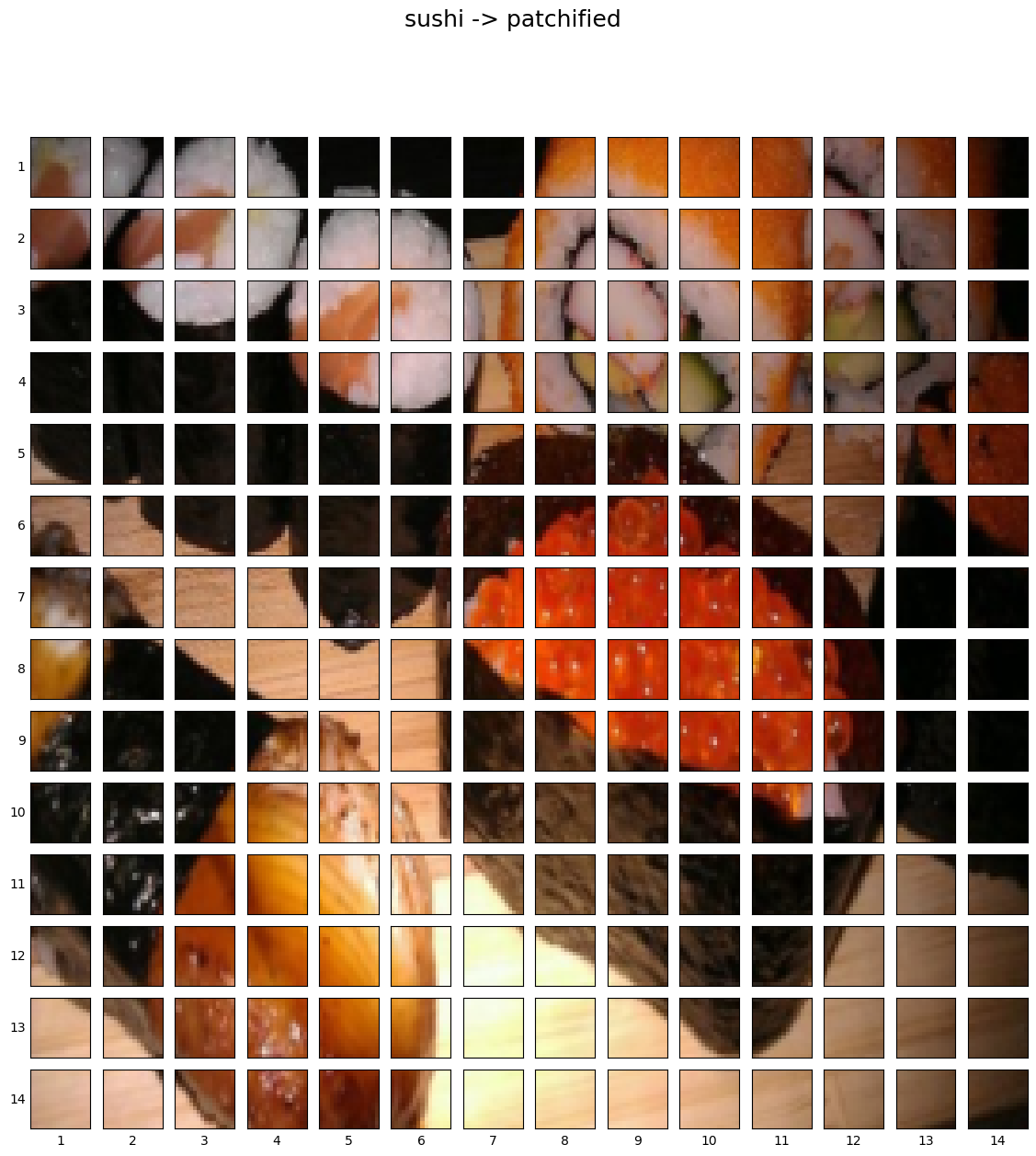
Original Image:
Number of parches per row: 14.0
Number of patches per column: 14.0
Patch size: 16 x 16 pixels
14*14 = 196 patches
- perhaps we could create the image patches and imge patch embedding ina single step using
torch.nn.Conv2d()and setting the kernel size and stride topatch_size.
- a convolutinal feature map is a laernable representation or
an embedding
#create conv2d layer to turn image into patches of learnable feature mas (embeddings))
from torch import nn
#set the patchpisze
patch_size = 16
#create a conv2d layers with hyperparameters from the ViT paper
conv2d = nn.Conv2d(in_channels=3,
                   out_channels=768, #D size from table 1 for ViT-Base, embedding size
                   kernel_size=patch_size,
                   stride=patch_size,
                   padding=0)
conv2d
Conv2d(3, 768, kernel_size=(16, 16), stride=(16, 16))
#paass the image thorugh the conv layer
image_out_of_conv = conv2d(image.unsqueeze(0)) #batchdimension  -> [batchsize, color channels, hieght, width]
print(image_out_of_conv.shape)
torch.Size([1, 768, 14, 14])
Now we've passed a single image into our conv2d layers we got
torch.Size([1, 768, 14, 14]) # [batchsize, embedding_dim, feature_map_height, feature_map_width]image_out_of_conv.requires_gradTrue
#plot random conv feature maps (embeddings)
import random
random_indexes = random.sample(range(0,768), k=5)
print(f"showing random convolutional feature maps from indexes: {random_indexes}")

# cretea a plot
fig, axis = plt.subplots(
    nrows=1,
    ncols=5,
    figsize=(12,12)
)

#plot rnadom image feature maps
for i, index in enumerate(random_indexes):
    image_conv_feature_map = image_out_of_conv[:, index, :, :]# index on the output tensor of the conv2d layer
    axis[i].imshow(image_conv_feature_map.squeeze().detach().numpy())#remove batch dim #remove from grad tracking/ switch to numpy for matplotlib
    axis[i].set(
        xticklabels=[],
        yticklabels=[],
        xticks=[],
        yticks=[]
    )
showing random convolutional feature maps from indexes: [683, 599, 74, 343, 635]
right now we've got a series of conv faeture maps (patch embeddings) that we want to flatten into a sequence of patch embeddings to satusfy the criteria of the ViT
print(f"{image_out_of_conv.shape} -> [batch_size, embeddingdim, feature_map_height, feature_map_width]")torch.Size([1, 768, 14, 14]) -> [batch_size, embeddingdim, feature_map_height, feature_map_width]
flatten_layer = nn.Flatten(start_dim=2,
                           end_dim=3)
flatten_layer(image_out_of_conv).shape #the order is still not w
torch.Size([1, 768, 196])
print(f"Originval image shape: {image.shape}")

#turn image into faeture maps
image_out_of_conv = conv2d(image.unsqueeze(0))#add batch dim
print(f"image feature map (patches) shape: {image_out_of_conv.shape}")

#flatten the faeture maps
image_out_of_conv_flattened = flatten_layer(image_out_of_conv)
print(f"Flattened image feature map shape : {image_out_of_conv_flattened.shape}")
Original image shape: torch.Size([3, 224, 224]) image feature map (patches) shape: torch.Size([1, 768, 14, 14]) Flattened image feature map shape : torch.Size([1, 768, 196]) torch.Size([1, 196, 768]) -> [batchsize, num of patches, embedding dimension]
we want this module to do a few things.
- Create a class called PatchEmbedding that inherits from nn.Module
- Initialize with appropriate hyperparameters, such a schannels, embedding dimension, patch_size.
- create a layer to turn an imamge into embedded patches using
nn.Conv2d(). - create a layer to flatten the feautre maps of the output of the layer in 3.
- define
forward()that defines the forward computations (eg. pass through layer from 3 to 4) - make sure the output shape of the layer reflects the required output shape of the patch embedding.
#1. create a class called Patchembedding
class PatchEmbedding(nn.Module):
    #2. initialize the layer owth appropriate hyperparamters
    def __init__(self,
                 in_channels: int=3,
                 patch_size: int=16,
                 embedding_dim: int=768): #from table 1 for ViT_base
        super().__init__()
        self.patch_size = patch_size
        #3. creata a layer to turn an image into embedded patches
        self.patcher = nn.Conv2d(in_channels=in_channels,
                                 out_channels=embedding_dim,
                                 kernel_size=patch_size,
                                 stride=patch_size,
                                 padding=0)
        #4. create a layer to flatten feature maps outputs of conv2d
        self.flatten = nn.Flatten(start_dim=2,
                                  end_dim=3)

    def forward(self, x:torch.Tensor) -> torch.Tensor:
        #creata assertion to mkae sure the image resolution is compatable with the patch size
        image_resolution = x.shape[-1]
        assert image_resolution % patch_size == 0, f"Input image size must be divisible by patchsize, image shape: {image_resolution}, patch_size = {self.patch_size}"

        #perfrm forawrd pass
        x_patched = self.patcher(x)
        x_flattened = self.flatten(x_patched)
        #6. make sure thereturned sequence embeddign dim are in the righ torder [batchsize,no of patches, embdedding dim]
        return x_flattened.permute(0,2,1)


patchify = PatchEmbedding(in_channels=3,
                          patch_size=16,
                          embedding_dim=768)
# pass a single image thorugh the patch embedding layer
print(f"input image size: {image.unsqueeze(0).shape}")
patch_embedded_image = patchify(image.unsqueeze(0)) # add an extra batchdim
print(f"output patch embedding sequence shape: {patch_embedded_image.shape}")
input image size: torch.Size([1, 3, 224, 224])
output patch embedding sequence shape: torch.Size([1, 196, 768])
- want to prepend a learnable class token to the start of the patch embedding
- in order to perform classificaiton we use the standard approach of adding an extra learnable classification token
patch_embedded_image.shapetorch.Size([1, 196, 768])
after we prepend the class token it should become [1,197, 768]
#get the batchsize and embedding dimension
batch_size = patch_embedded_image.shape[0]
embedding_dimension = patch_embedded_image.shape[-1]
batch_size, embedding_dimension

#create class token embedding as a laernable paramter that shares the same size as the embedding dimension (D)
class_token = nn.Parameter(torch.ones(batch_size, 1, embedding_dimension),
                           requires_grad=True)  # to make the paramter learnable its on by default
class_token.shape
torch.Size([1, 1, 768])
patch_embedded_image.shapetorch.Size([1, 196, 768])
#add the class token embedding to the from of the patch embedding # From the paper
patch_embedded_image_with_class_embedding= torch.cat((class_token, patch_embedded_image),
                                                     dim=1) #no of patches dim
print(f"{patch_embedded_image_with_class_embedding.shape} -> batch_size, class_token + no_of_patches, embedding_dim")
torch.Size([1, 197, 768]) -> batch_size, class_token + no_of_patches, embedding_dim
patch_embedded_image_with_class_embeddingtensor([[[ 1.0000, 1.0000, 1.0000, ..., 1.0000, 1.0000, 1.0000],
[-0.2044, 0.1213, -0.3727, ..., -0.0422, -0.1065, -0.1086],
[-0.1035, -0.0072, -0.4738, ..., -0.0445, -0.1931, 0.1067],
...,
[-0.2448, 0.0557, -0.5102, ..., -0.0727, -0.2336, -0.0618],
[-0.1278, 0.0315, -0.3228, ..., -0.0731, -0.1883, -0.0347],
[-0.0428, 0.0037, -0.1469, ..., -0.0665, -0.0937, -0.0178]]],
grad_fn=)
want to: create a series of 1d learnable positionembedding and to add them to the sequence of patch embeddings
#view the sequence of patch embeddinigs withthe prepended class embeddings
patch_embedded_image_with_class_embedding, patch_embedded_image_with_class_embedding.shape
(tensor([[[ 1.0000, 1.0000, 1.0000, ..., 1.0000, 1.0000, 1.0000],
[-0.2044, 0.1213, -0.3727, ..., -0.0422, -0.1065, -0.1086],
[-0.1035, -0.0072, -0.4738, ..., -0.0445, -0.1931, 0.1067],
...,
[-0.2448, 0.0557, -0.5102, ..., -0.0727, -0.2336, -0.0618],
[-0.1278, 0.0315, -0.3228, ..., -0.0731, -0.1883, -0.0347],
[-0.0428, 0.0037, -0.1469, ..., -0.0665, -0.0937, -0.0178]]],
grad_fn=),
torch.Size([1, 197, 768]))
 #calculate the N no of  patches
num_patches = int((height * width) / patch_size**2)
#get the embedding dimension
embedding_dimension = patch_embedded_image_with_class_embedding.shape[-1]
embedding_dimension

#create the learnable 1D position embedding
position_embedding = nn.Parameter(torch.ones(batch_size, #batchsize or 1
                                             num_patches+1, #from paper # and as we added the class token  we get 197 instead of 196
                                             embedding_dimension),
                                  requires_grad=True) #learnable so it gets updated during training
position_embedding, position_embedding.shape
(Parameter containing:
tensor([[[1., 1., 1., ..., 1., 1., 1.],
[1., 1., 1., ..., 1., 1., 1.],
[1., 1., 1., ..., 1., 1., 1.],
...,
[1., 1., 1., ..., 1., 1., 1.],
[1., 1., 1., ..., 1., 1., 1.],
[1., 1., 1., ..., 1., 1., 1.]]], requires_grad=True),
torch.Size([1, 197, 768]))
Add the position embedding to the patch and class token embeddding
patch_embedded_image_with_class_embedding, patch_embedded_image_with_class_embedding.shape (tensor([[[ 1.0000, 1.0000, 1.0000, ..., 1.0000, 1.0000, 1.0000],
[-0.2044, 0.1213, -0.3727, ..., -0.0422, -0.1065, -0.1086],
[-0.1035, -0.0072, -0.4738, ..., -0.0445, -0.1931, 0.1067],
...,
[-0.2448, 0.0557, -0.5102, ..., -0.0727, -0.2336, -0.0618],
[-0.1278, 0.0315, -0.3228, ..., -0.0731, -0.1883, -0.0347],
[-0.0428, 0.0037, -0.1469, ..., -0.0665, -0.0937, -0.0178]]],
grad_fn=),
torch.Size([1, 197, 768]))
patch_and_position_embedding = patch_embedded_image_with_class_embedding + position_embedding
patch_and_position_embedding, patch_and_position_embedding.shape
(tensor([[[2.0000, 2.0000, 2.0000, ..., 2.0000, 2.0000, 2.0000],
[0.7956, 1.1213, 0.6273, ..., 0.9578, 0.8935, 0.8914],
[0.8965, 0.9928, 0.5262, ..., 0.9555, 0.8069, 1.1067],
...,
[0.7552, 1.0557, 0.4898, ..., 0.9273, 0.7664, 0.9382],
[0.8722, 1.0315, 0.6772, ..., 0.9269, 0.8117, 0.9653],
[0.9572, 1.0037, 0.8531, ..., 0.9335, 0.9063, 0.9822]]],
grad_fn=),
torch.Size([1, 197, 768]))
import helper_functions
#set the seeds
helper_functions.set_seeds()

#!set the patch ize: there are multiple patchsizes in the paper we use 16
patch_size = 16

#2. print the sahapes of the original image and get the image dimensions
print(f"Image tensor shape: {image.shape}")
height, width = image.shape[1], image.shape[2]

#3. get the image tensor and add a batch dimension
x = image.unsqueeze(0)
print(f"Input image shape: {x.shape}")

#4.create a patch embedding layer
patch_embedding_layer = PatchEmbedding(in_channels=3,
                                       patch_size=patch_size,
                                       embedding_dim=768) #inline with ViT-base in table 1
#5. pass input iamge through patchembedding layer
patch_embedding = patch_embedding_layer(x)
print(f"Patch embedding shape: {patch_embedding.shape}")
#6.creating class token embedding
batch_size = patch_embedding.shape[0]
embedding_dimension = patch_embedding.shape[-1]
class_token = nn.Parameter(torch.ones(batch_size,1,embedding_dimension), #using ones for laerning use randn for practical architecture
                          requires_grad=True)
print(f"class token embedding shape: {class_token.shape}")
#7. prepend the class token embedding to the patch embedding
patch_embedding_class_token = torch.cat((class_token, patch_embedding), dim=1)
print(f"patch_embedding with class token shape :{patch_embedding_class_token.shape}")
#8.create position embedding
number_of_patches = int((height*width) / patch_size**2)
position_embedding = nn.Parameter(torch.ones(1, number_of_patches+1, embedding_dimension),
                                  requires_grad=True) #look at paper for plus 1
#9. add the posotion embedding to patch embedding with class otken
patch_and_position_embedding = patch_embedding_class_token + position_embedding
print(f"patch_and_position_embedding shape: {patch_and_position_embedding.shape}")
Image tensor shape: torch.Size([3, 224, 224])
Input image shape: torch.Size([1, 3, 224, 224])
Patch embedding shape: torch.Size([1, 196, 768])
class token embedding shape: torch.Size([1, 1, 768])
patch_embedding with class token shape :torch.Size([1, 197, 768])
patch_and_position_embedding shape: torch.Size([1, 197, 768])
- consists of 2 main blocks of eq.2 and eq.3
- for many of these layers like
MSApytorch has prebuilt function for the layer
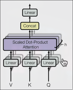
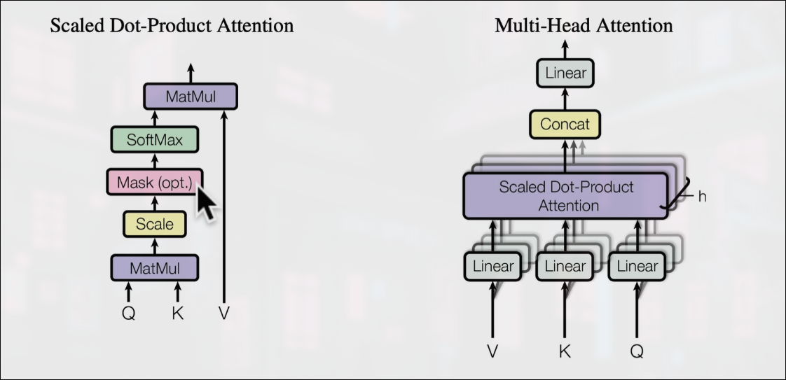
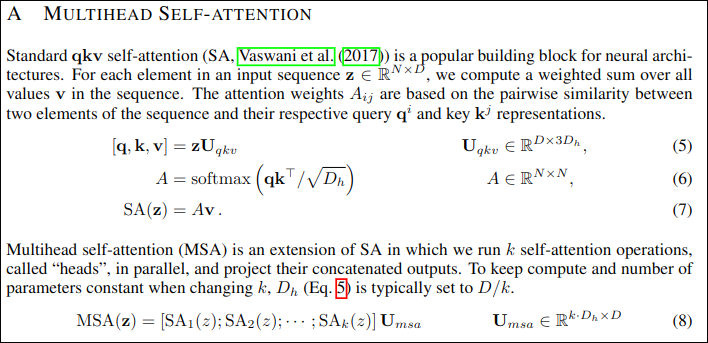
Q- Query, K-key, V-value are instances of the same sequence of vectors,
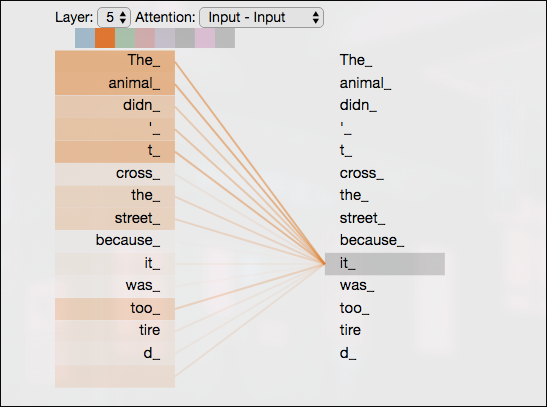
tells us which patch needs to pay how much attention to which other word or image patch in the same vector,
to find how much related 1 patch is to another
-
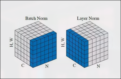
  - normalization technique to normalize the distributions of the intermediate layers,

  - it enables smoother gradients, faster training, and better generalization accuracy
- Normalization - make everything have name mean and same std deviation
- mean and std dev are calculated over the last D dimension, where D is the dim of normalized shape
- when we normalize along the embedding dimension, it's like making all of the steps in the staircase to the same size
in docs:
- no of patches = sequence
- features = embedding dimension
## creating a multihead self attentionlayer in pytorch
class MultiHeadSelfAttentionBlock(nn.Module):
    """creates a multihead self attention block (MSA block)
    """
    def __init__(self,
                 embedding_dimension: int=768, #Hidden size D (embedding dimension) from table 1 for ViT _base
                 num_heads: int=12, #heads from table 1 for ViTbase
                 attn_dropout: int=0):#dropout is only used for dense layer/ fully coneccted/ linaer/ feed forward. but not for QKV projections
                                        #ie we are not gonna use dropout for our MSA block
        super().__init__()
    #create the norm layer (LN)
        self.layer_norm = nn.LayerNorm(
            normalized_shape=embedding_dimension#check pytroch docs
        )

        self.multihead_attn = nn.MultiheadAttention(
            embed_dim=embedding_dimension, # hidden size D (embedding dimension) from table 1 for ViT-base
            num_heads=num_heads, #no of MSA heads
            dropout=attn_dropout, #zero
            batch_first=True #batch_first – If True, then the input and output tensors are provided as (batch, no of patches or sequence, features or embedding dimension). Default: False (seq, batch, feature) #from pytorch docs
        )

    def forward(self, x: torch.Tensor) -> torch.Tensor: # Q,K and V are x: they are different instances of the same vector
        x = self.layer_norm(x)
        attn_output, _ =  self.multihead_attn(query=x,
                                                key=x,
                                                value=x,
                                                need_weights=False)                  # u can also get attn_weights ie weights of the attention layer #check the docs.
        return attn_output
# create an instance MSA block
multihead_self_attention_block = MultiHeadSelfAttentionBlock(
embedding_dimension=768,
num_heads=12,
attn_dropout=0
)
#pass the patch and position image embedding sequence thourgh our MSA Block
patched_image_through_msa_block = multihead_self_attention_block(patch_and_position_embedding)
print(f"Input shape of MSA bock: {patch_and_position_embedding.shape}")
print(f"Output shape of MSA block; {patched_image_through_msa_block.shape}")Input shape of MSA bock: torch.Size([1, 197, 768]) Output shape of MSA block; torch.Size([1, 197, 768])
patch_and_position_embedding tensor([[[2.0000, 2.0000, 2.0000, ..., 2.0000, 2.0000, 2.0000],
[0.4842, 1.1071, 0.9806, ..., 1.2911, 0.8060, 1.1216],
[0.4619, 0.9047, 0.8579, ..., 1.3663, 0.9612, 1.4155],
...,
[0.4886, 1.0627, 0.8966, ..., 1.3370, 0.7364, 1.2223],
[0.6908, 1.0200, 0.9475, ..., 1.2131, 0.8064, 1.1861],
[0.8316, 1.0010, 0.9662, ..., 1.0398, 0.9115, 1.1034]]],
grad_fn=)
#output
patched_image_through_msa_block
tensor([[[-0.1992, -0.1785, 0.0754, ..., -0.3689, 0.8296, -0.4426],
[-0.1836, -0.1788, 0.0768, ..., -0.3568, 0.8418, -0.4648],
[-0.1715, -0.1662, 0.0784, ..., -0.3658, 0.8433, -0.4552],
...,
[-0.1745, -0.1771, 0.0726, ..., -0.3638, 0.8436, -0.4722],
[-0.1707, -0.1792, 0.0704, ..., -0.3669, 0.8461, -0.4732],
[-0.1732, -0.1884, 0.0665, ..., -0.3622, 0.8442, -0.4701]]],
grad_fn=)
patched_image_through_msa_block == patch_and_position_embeddingtensor([[[False, False, False, ..., False, False, False],
[False, False, False, ..., False, False, False],
[False, False, False, ..., False, False, False],
...,
[False, False, False, ..., False, False, False],
[False, False, False, ..., False, False, False],
[False, False, False, ..., False, False, False]]])
* MLP = a quite broad term for a block with a series of layer(s), ayers can be multiple or even only one hidden layer.
* layers can mean: fully connected/ dense/ linear/ feed-forward, all are often similar names for the same thing.
In pytorch theyre called `torch.nn.Linear`.
In tensorflow theyre called `tf.keras.dense
MLP_size / number of hidden units of MLP = 3072 for ViT-Base (from table 1)
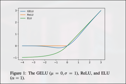
* the standard Gaussian cumulative distribution function. The GELU nonlinearity weights inputs by their percentile, rather than gates inputs by their sign as in ReLUs ().
* Consequently the GELU can be thought of as a smoother ReLU.
* applies the Gaussin Error Linear Units Functions (GELU)
Dropout is applied after every linear layer in MLP
* value for dropout is available at table 3 Dropout = 0.1 for Vit/b-16
In pseudocode:
#MLP block
x = layer norm -> linear layer -> non-linear layer -> dropout -> linear layer -> dropout
class MLPBlock(nn.Module):
def __init__(self,
embedding_dim: int=768,
mlp_size: int=3072,
dropout: float=0.1
):
super().__init__()
#creat the norm layer (LN)
self.layer_norm = nn.LayerNorm(
normalized_shape=embedding_dim
)
#creat eh MLP
self.mlp = nn.Sequential(
nn.Linear(in_features=embedding_dim,
out_features=mlp_size), #project to a larger size # to hopfully capture some fore information
nn.GELU(),
nn.Dropout(
p=dropout
),
nn.Linear(in_features=mlp_size,
out_features=embedding_dim), #squeeze it back to the embedding dimension
nn.Dropout(
p=dropout
)
)
def forward(self, x: torch.Tensor) -> torch.Tensor:
x = self.layer_norm(x)
x = self.mlp(x)
return x
#return self.mlp(self.layer_norm(x) #same as above# this will benefit from operator fusion side track: https://horace.io/brrr_intro.html || checkout torch.compile feature that leverages operator fusion mentioned above
#create an instance of MLP block
mlp_block = MLPBlock(embedding_dim=768, #talble 1 value
                     mlp_size=3072, #table 1 value
                     dropout=0.1) #table 3 value

#pass ouot through the MLP block
patched_image_through_mlp_block = mlp_block(patched_image_through_msa_block)
print(f"Input shape of the MLP block: {patched_image_through_msa_block.shape}")
print(f"Output shape of the  MLP blcok: {patched_image_through_mlp_block.shape}")
Input shape of the MLP block: torch.Size([1, 197, 768])
Output shape of the MLP blcok: torch.Size([1, 197, 768])
#the variables have changed even though the values are the same
patched_image_through_mlp_block == patched_image_through_msa_block
tensor([[[False, False, False, ..., False, False, False],
[False, False, False, ..., False, False, False],
[False, False, False, ..., False, False, False],
...,
[False, False, False, ..., False, False, False],
[False, False, False, ..., False, False, False],
[False, False, False, ..., False, False, False]]])
this is not really the correct order of doing things as we havent added the residual connections yet
The transfformer encoder is a combination of alternating blocks of MSA blocks and MLP blocks LN is applied between every block, and residual connections after every block
encoder = turn a sequence into a laernable representation
decoder = turna learnable representation to some sort of sequence
encoders in NLP converts text(sequence) into numbers decoders decontructs encoded numbers into text (sequence) (in a translator)
seq2seq is a ml model usually used in NLP. This is also where our transformer came from ie NLP which has encoders as well as decoders
thats were our name transformer encoder comes from,
since our goal is image classification instead of a decoder we use an MLP instead of an Decoder
- residual connnections = add alyer(s) input to its subsequent output,
this enables the creation of deeper networks (prevents weights from getting too small ie preventing spare networks or vanishing gradient problem)
In pseudo:
#transfomer encoder:
x_input (output/sequence of embedding patches) -> MSA_Block -> [MSA_Block + x_input (residual)] -> MLP_Block -> [MLP_block_output + (MSA_block_output + x_input) ] -> ...class TransformerEncoderBlock(nn.Module):
"""creates a transformer block instance"""
def __init__(self,
embedding_dim:int=768, # hidden size D from Table 1 for ViT-Base
num_heads:int=12, # heads from Table 1 for ViT-Base
mlp_size:int=3072, # MLP size from Table 1 for ViT-Base
mlp_dropout:float=0.1, # dropout for dense layers from Table 3 for ViT-Base
attn_dropout:float=0): # dropout for attention layers
super().__init__()
# 3. Create MSA block (equation 2)
self.msa_block = MultiHeadSelfAttentionBlock(embedding_dimension=embedding_dim,
num_heads=num_heads,
attn_dropout=attn_dropout)
# 4. Create MLP block (equation 3)
self.mlp_block = MLPBlock(embedding_dim=embedding_dim,
mlp_size=mlp_size,
dropout=mlp_dropout)
# 5. Create a forward() method
def forward(self, x:torch.Tensor) -> torch.Tensor:
# 6. Create residual connection for MSA block (add the input to the output)
x = self.msa_block(x) + x
# 7. Create residual connection for MLP block (add the input to the output)
x = self.mlp_block(x) + x
return x#create an instance of TransformerEncoderBlock()
transformer_encoder_block = TransformerEncoderBlock()
transformer_encoder_blockTransformerEncoderBlock(
(msa_block): MultiHeadSelfAttentionBlock(
(layer_norm): LayerNorm((768,), eps=1e-05, elementwise_affine=True)
(multihead_attn): MultiheadAttention(
(out_proj): NonDynamicallyQuantizableLinear(in_features=768, out_features=768, bias=True)
)
)
(mlp_block): MLPBlock(
(layer_norm): LayerNorm((768,), eps=1e-05, elementwise_affine=True)
(mlp): Sequential(
(0): Linear(in_features=768, out_features=3072, bias=True)
(1): GELU(approximate='none')
(2): Dropout(p=0.1, inplace=False)
(3): Linear(in_features=3072, out_features=768, bias=True)
(4): Dropout(p=0.1, inplace=False)
)
)
)
rand_tensor = torch.randn(size=(1,197,768))
transformer_encoder_block(rand_tensor).shape

from torchinfo import summary

summary(model=transformer_encoder_block,
        input_size=(1,197,768), #<- the size of the output of the embedded patches and NOT the original image size
        col_names=["input_size", 'output_size', 'num_params', 'trainable'],
        col_width=20,
        row_settings=['var_names'])
================================================================================================================================== Layer (type (var_name)) Input Shape Output Shape Param # Trainable ================================================================================================================================== TransformerEncoderBlock (TransformerEncoderBlock) [1, 197, 768] [1, 197, 768] -- True ├─MultiHeadSelfAttentionBlock (msa_block) [1, 197, 768] [1, 197, 768] -- True │ └─LayerNorm (layer_norm) [1, 197, 768] [1, 197, 768] 1,536 True │ └─MultiheadAttention (multihead_attn) -- [1, 197, 768] 2,362,368 True ├─MLPBlock (mlp_block) [1, 197, 768] [1, 197, 768] -- True │ └─LayerNorm (layer_norm) [1, 197, 768] [1, 197, 768] 1,536 True │ └─Sequential (mlp) [1, 197, 768] [1, 197, 768] -- True │ │ └─Linear (0) [1, 197, 768] [1, 197, 3072] 2,362,368 True │ │ └─GELU (1) [1, 197, 3072] [1, 197, 3072] -- -- │ │ └─Dropout (2) [1, 197, 3072] [1, 197, 3072] -- -- │ │ └─Linear (3) [1, 197, 3072] [1, 197, 768] 2,360,064 True │ │ └─Dropout (4) [1, 197, 768] [1, 197, 768] -- -- ================================================================================================================================== Total params: 7,087,872 Trainable params: 7,087,872 Non-trainable params: 0 Total mult-adds (M): 4.73 ================================================================================================================================== Input size (MB): 0.61 Forward/backward pass size (MB): 8.47 Params size (MB): 18.90 Estimated Total Size (MB): 27.98 ==================================================================================================================================
as u can see it expands in the MLP layer then compresses back, might be able to identify more features
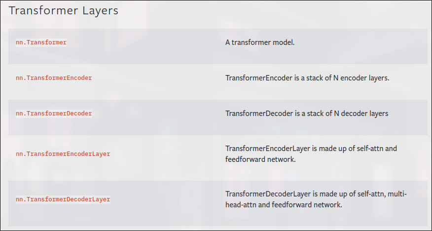
since how good the transformer arch is, pytorch has implemented ready to use transformer encoder layers
#create the same as above with torch.nn.TransformerEncoderLayer()
torch_transformer_encoder_layer = nn.TransformerEncoderLayer(d_model=768,# embedding dimension/size from table 1
                                                             nhead=12, #no of heads from table 1
                                                             dim_feedforward=3072, # MLP size from table 1
                                                             dropout=0.1, #fro table 3
                                                             activation='gelu',
                                                             batch_first=True,
                                                             norm_first=True # Layer Norm is First if True, default is false
                                                             )
# this is implementing Eq2 and eq3 at the same time
torch_transformer_encoder_layer
TransformerEncoderLayer(
(self_attn): MultiheadAttention(
(out_proj): NonDynamicallyQuantizableLinear(in_features=768, out_features=768, bias=True)
)
(linear1): Linear(in_features=768, out_features=3072, bias=True)
(dropout): Dropout(p=0.1, inplace=False)
(linear2): Linear(in_features=3072, out_features=768, bias=True)
(norm1): LayerNorm((768,), eps=1e-05, elementwise_affine=True)
(norm2): LayerNorm((768,), eps=1e-05, elementwise_affine=True)
(dropout1): Dropout(p=0.1, inplace=False)
(dropout2): Dropout(p=0.1, inplace=False)
)
summary(model=torch_transformer_encoder_layer,
        input_size=(1,197,768), #<- the size of the output of the embedded patches and NOT the original image size
        col_names=["input_size", 'output_size', 'num_params', 'trainable'],
        col_width=20,
        row_settings=['var_names'])
================================================================================================================================== Layer (type (var_name)) Input Shape Output Shape Param # Trainable ================================================================================================================================== TransformerEncoderLayer (TransformerEncoderLayer) [1, 197, 768] [1, 197, 768] 7,087,872 True ================================================================================================================================== Total params: 7,087,872 Trainable params: 7,087,872 Non-trainable params: 0 Total mult-adds (M): 0.00 ================================================================================================================================== Input size (MB): 0.61 Forward/backward pass size (MB): 0.00 Params size (MB): 0.00 Estimated Total Size (MB): 0.61 ==================================================================================================================================
The output of the summary is slightly different to ours due to how torch.nn.TransformerEncoderLayer() constructs its layer.
But the layers it uses, number of parameters and input and output shapes are the same.
Less prone to errors - Generally, if a layer makes it into the PyTorch standard library, its been tested and tried to work.
Potentially better performance - as of now, the PyTorch implemented version of torch.nn.TransformerEncoderLayer() can see a speedup of more than 2x on many common workloads.
they generally have a smaller forward/backward pass size
then why did we spend all the time recreating the encoder piece by piece instead of just using the inbuilt function? to know how things work in the background and practise
#create a ViT class
class ViT(nn.Module):
    def __init__(self,
                 img_size:int=224, #table 3 from the ViT paper
                 in_channels:int=3, #as were dealing with colored images
                 patch_size:int=16,# need patchsze to be compatible with img_size (add assetion)
                 num_transformer_layers:int=12,#heads / transformer layerstable 1 for layers in ViT_base
                 embedding_dimension:int=768, #hidden_size D from table 1 for ViTBase
                 mlp_size:int=3072, #mlp hidden unit size table 1
                 attn_dropout:int=0,
                 mlp_dropout:float=0.1,
                 embedding_dropout:float=0.1, #dropout for patch and position embedddings #check experiment details B.!
                 num_classes:int=1000 #num of classes in our classification problem #set to a 1000 as original ViT was trained on imagenet
                 ):
        super().__init__()

        #make an assertion to check if image size is compatible witht he patchsize
        assert img_size % patch_size == 0, f"Image size must be divisble by patch size, img_size: {img_size}, patch_size {patch_size}"

        #calc the no o fpaches (height * width / patch_size **2)
        self.num_patches = (img_size * img_size)// patch_size**2 #HW/PP make sure you have // to floor

        #create learnable class embedding #needs to go at front of seqience of patch embeddings
        self.class_embedding = nn.Parameter(data=torch.randn(1, 1, embedding_dimension), #remeber we made it with torch.ones before? now its randn
                                            requires_grad=True) #make it trainable ie update params with optimizer

        #create learning position embedding
        self.position_embeddding = nn.Parameter(data=torch.randn(1, self.num_patches+1, embedding_dimension))

        #cerae embedding dorpout value
        self.embedding_dropout = nn.Dropout(p=embedding_dropout)

        #create create patch_embedding_layer
        self.patch_embedding = PatchEmbedding(in_channels=in_channels,
                                              patch_size=patch_size,
                                              embedding_dim=embedding_dimension)
        # you can probably modularity this previous block and amke it much easier to create a patch embedding layer

        #crete the transformer encoder block
        #to stack 12 of them on top of eaceh oterh in a manual way
        self.transformer_encoder = nn.Sequential(*[TransformerEncoderBlock(embedding_dim=embedding_dimension,
                                                                           num_heads=num_transformer_layers,
                                                                           mlp_size=mlp_size,
                                                                           mlp_dropout=mlp_dropout) for _ in range(num_transformer_layers)]) # '*' means all of the layers in this comprehension that gets turned into a sequential block

        #create classifier head
        self.classifier = nn.Sequential(
            nn.LayerNorm(normalized_shape=embedding_dimension),
            nn.Linear(in_features=embedding_dimension, #becaus ethe output of the transformerencodinng block is going to have  adim size of embedding dim
                      out_features=num_classes) #since this the final output layer we need out features equal to the number of classes
        )


    def forward(self, x:torch.Tensor) -> torch.Tensor:
        #EQUATION 1
        #get the batch)size
        batch_size = x.shape[0] #why hardcore when manipulate the data

        #unlike in the paper we arent using 4096 batch_size because of hardware limitations
        #create class token embedding and expand it to match the batch_size ( equation 1)
        class_token = self.class_embedding.expand(batch_size, -1, -1) # "-1" means to infer the dimension #check cell below

        #create patch_embedding
        x = self.patch_embedding(x)

        #concat class token embedding and patch_embedding
        x = torch.concat((class_token, x), dim=1) #(batchsize, no of patches, embedding_dim)

        #add the position embeddding to class token and patch_embedding
        x = self.position_embeddding + x

        #Run embedding dropout # when used is applied after every linear layer expect KQV projects /output ie MSA projections
        #and directly after adding positional to patch embeddings: from EXPERMENT DETAILS B.1
        x = self.embedding_dropout(x)

        #EQUATION 2 AND 3
        #pass our position and patch_embedding into our transformer encoder
        x = self.transformer_encoder(x)

        #EQUATION 4
        #put 0th index logit through the classifier
        x = self.classifier(x[:, 0]) # every batch, and the zeroth index

        return x
batch_size = 32
embedding_dimension = 768
class_embedding = nn.Parameter(data=torch.randn(1, 1, embedding_dimension), #remeber we made it with torch.ones before? now its randn
requires_grad=True) #make it trainable ie update params with optimizer
class_embedding_expanded = class_embedding.expand(batch_size, -1, -1) #"-1" means to infer the dimensions
class_embedding.shape, class_embedding_expanded.shape
#we've expanded thhe class_token embedding across every image in a batch(torch.Size([1, 1, 768]), torch.Size([32, 1, 768]))
u can see we only want to pass the classification token as it says (z^0 L) [z zeroth of the last token]
this is why the figure has an arrow only on the last token here at the classification token, ie we only want to pass the classicatino token into the MLP head
- "the classficaiton head is implemeneted by a MLP iwth one hidden layer at pre-training time and by a single linear layer at fine-tuning time"
note: oddly enough the equation 4 doesnt mention an MLP layer, but the presence of an MLP layer at the end is implied throughout the paper
vit = ViT()
vit
ViT(
(embedding_dropout): Dropout(p=0.1, inplace=False)
(patch_embedding): PatchEmbedding(
(patcher): Conv2d(3, 768, kernel_size=(16, 16), stride=(16, 16))
(flatten): Flatten(start_dim=2, end_dim=3)
)
(transformer_encoder): Sequential(
(0): TransformerEncoderBlock(
(msa_block): MultiHeadSelfAttentionBlock(
(layer_norm): LayerNorm((768,), eps=1e-05, elementwise_affine=True)
(multihead_attn): MultiheadAttention(
(out_proj): NonDynamicallyQuantizableLinear(in_features=768, out_features=768, bias=True)
)
)
(mlp_block): MLPBlock(
(layer_norm): LayerNorm((768,), eps=1e-05, elementwise_affine=True)
(mlp): Sequential(
(0): Linear(in_features=768, out_features=3072, bias=True)
(1): GELU(approximate='none')
(2): Dropout(p=0.1, inplace=False)
(3): Linear(in_features=3072, out_features=768, bias=True)
(4): Dropout(p=0.1, inplace=False)
)
)
)
...
(classifier): Sequential(
(0): LayerNorm((768,), eps=1e-05, elementwise_affine=True)
(1): Linear(in_features=768, out_features=1000, bias=True)
)
)
beautiful.
helper_functions.set_seeds()

#create a random image tensor with same shape as asingle image
random_image_tensor = torch.randn(size=(1,3,224,224))

#create a instace of ViT with the no of class we're working with (pizza, steak and sushi) ie 3
vit = ViT(num_classes=len(class_names))

#pass the random tensor though our vit instance
vit_output = vit(random_image_tensor)
vit_output, vit_output.shape
(tensor([[-0.2377, 0.7360, 1.2137]], grad_fn=),
torch.Size([1, 3]))
 summary(model=ViT(num_classes=len(class_names)),
        input_size=(1,3, 224, 224), #<- [B,C,H,W]
        col_names=["input_size", 'output_size', 'num_params', 'trainable'],
        col_width=20,
        row_settings=['var_names'])
============================================================================================================================================ Layer (type (var_name)) Input Shape Output Shape Param # Trainable ============================================================================================================================================ ViT (ViT) [1, 3, 224, 224] [1, 3] 152,064 True ├─PatchEmbedding (patch_embedding) [1, 3, 224, 224] [1, 196, 768] -- True │ └─Conv2d (patcher) [1, 3, 224, 224] [1, 768, 14, 14] 590,592 True │ └─Flatten (flatten) [1, 768, 14, 14] [1, 768, 196] -- -- ├─Dropout (embedding_dropout) [1, 197, 768] [1, 197, 768] -- -- ├─Sequential (transformer_encoder) [1, 197, 768] [1, 197, 768] -- True │ └─TransformerEncoderBlock (0) [1, 197, 768] [1, 197, 768] -- True │ │ └─MultiHeadSelfAttentionBlock (msa_block) [1, 197, 768] [1, 197, 768] 2,363,904 True │ │ └─MLPBlock (mlp_block) [1, 197, 768] [1, 197, 768] 4,723,968 True ... │ └─TransformerEncoderBlock (11) [1, 197, 768] [1, 197, 768] -- True │ │ └─MultiHeadSelfAttentionBlock (msa_block) [1, 197, 768] [1, 197, 768] 2,363,904 True │ │ └─MLPBlock (mlp_block) [1, 197, 768] [1, 197, 768] 4,723,968 True ├─Sequential (classifier) [1, 768] [1, 3] -- True │ └─LayerNorm (0) [1, 768] [1, 768] 1,536 True │ └─Linear (1) [1, 768] [1, 3] 2,307 True ============================================================================================================================================ Total params: 85,800,963 Trainable params: 85,800,963 Non-trainable params: 0 Total mult-adds (M): 172.47 ============================================================================================================================================ Input size (MB): 0.60 Forward/backward pass size (MB): 102.88 Params size (MB): 229.20 Estimated Total Size (MB): 332.69 ============================================================================================================================================
Now that we've replicated the architecture, lets see how it perofmrs on our data
- adam optimizer
- beta1 = 0.9; beta2 = 0.999 (defaults)
- weight_decay = 0.1 (high) weight decay is L2 regularization method by addning a small penalty, usually the square of the weights, (all the weights of the model), to the loss function, therefore larger weights are penalized more than smaller weights, preventing sparse networks caused in L1 regularization where the absolute sum of the weights are added to the loss, which makes weights tend to 0.0 making it sparse. Regularization prevents overfitting.
- base learning rate =
$10^-3$ from table 3
#optimizer
optimizer = torch.optim.Adam(params=vit.parameters(),
                            betas=(0.9,0.999),
lr=1e-3) #from table 3the vit paper doesnt mention what loss function they used.
therefore since it is a multi-clas classification we'll use nn.crossentropyloss
# loss
loss_fn = nn.CrossEntropyLoss()from pytorch_modules.modules import train_engine
results = train_engine.train(model=vit,
train_dataloader=train_dataloader,
test_dataloader=test_dataloader,
optimizer=optimizer,
loss_fn=loss_fn,
epochs=10,
device=device)Because training in kaggle was faster:
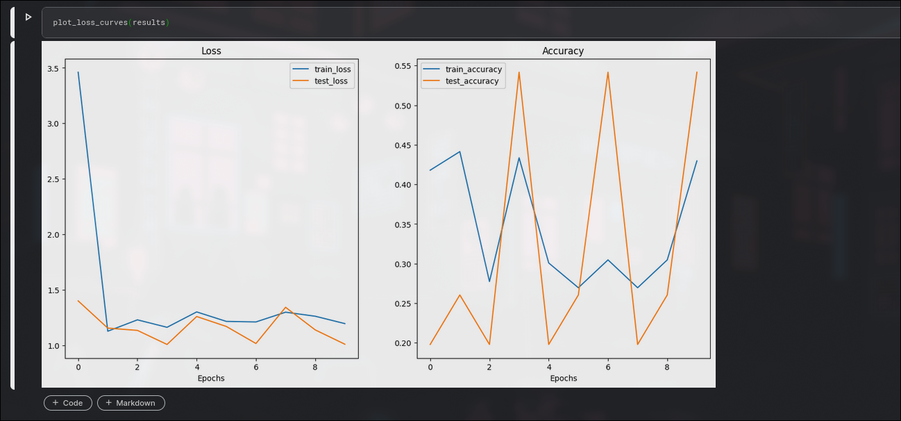
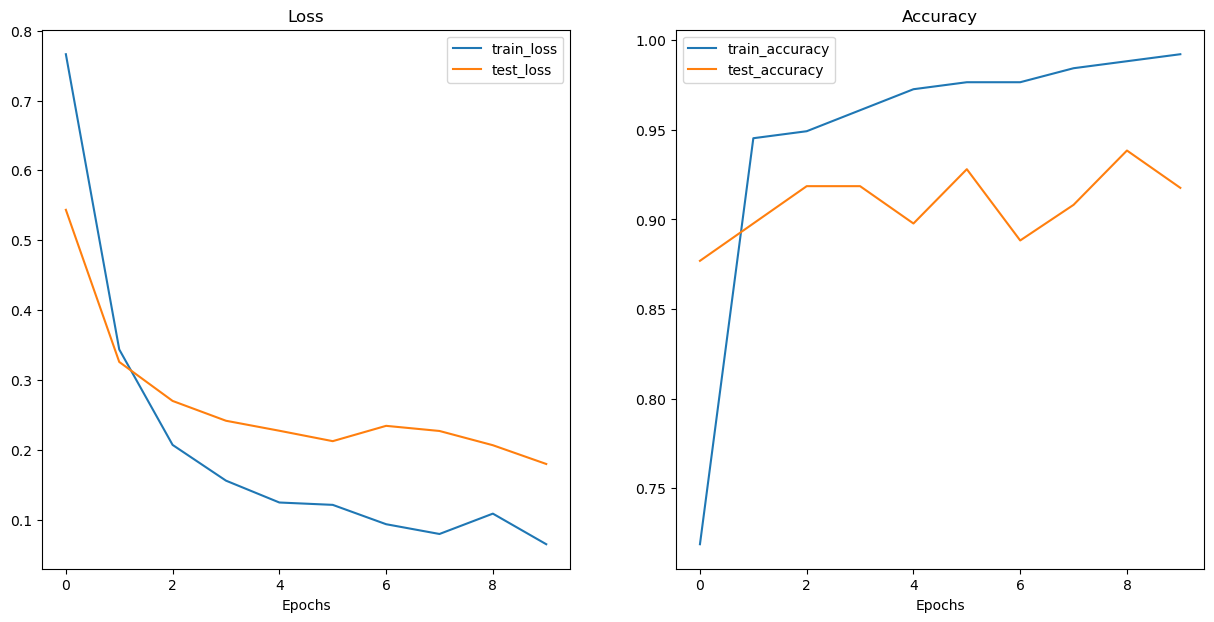
plotting loss curves:
We've replicated the model architecture correctly, but what was different our training procedure to get poor results and vit papers training procedure to have great results
The original ViT model simply had gargantuous amounts of data, which gave it more options to learn, and transformers are known for their data hungry training because of how "general" they are. In deep learning more data is ALWAYS a good thing
| Hyperparameter value | ViT Paper | Our implementation |
|---|---|---|
| Number of training images | 1.3M (ImageNet-1k), 14M (ImageNet-21k), 303M (JFT) | 225 |
| Epochs | 7 (for largest dataset), 90, 300 (for ImageNet) | 10 |
| Batch size | 4096 | 32 |
| Learning rate warmup | 10k steps (Table 3) | None |
| Learning rate decay | Linear/Cosine (Table 3) | None |
| Gradient clipping | Global norm 1 (Table 3) | None |
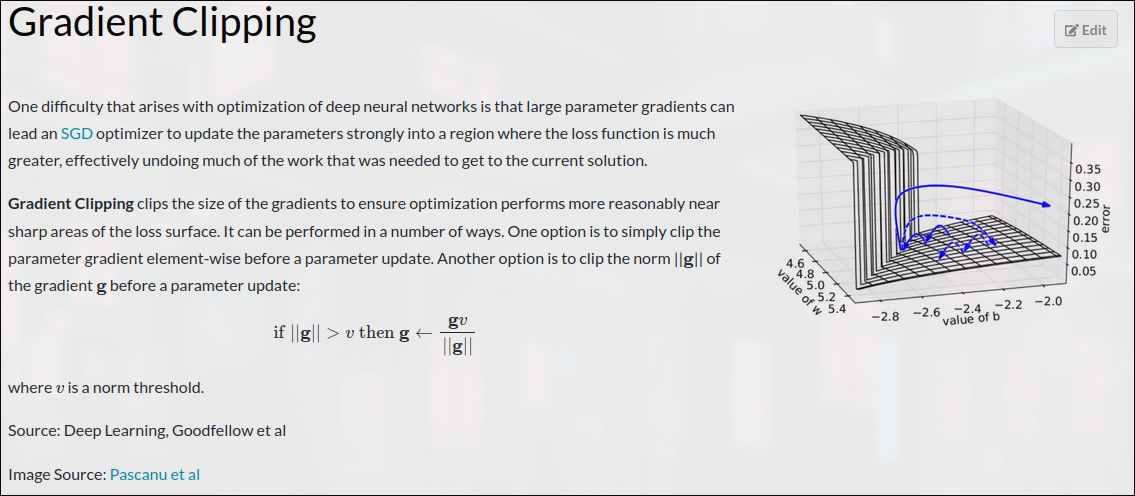
learning rate warmup, learning rate decay and gradient clipping are used as regularization techniques to reduce overfitting
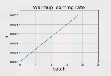
Linear Warmup is a learning rate schedule where we linearly increase the learning rate from a low rate to a constant rate thereafter. This reduces volatility in the early stages of training.
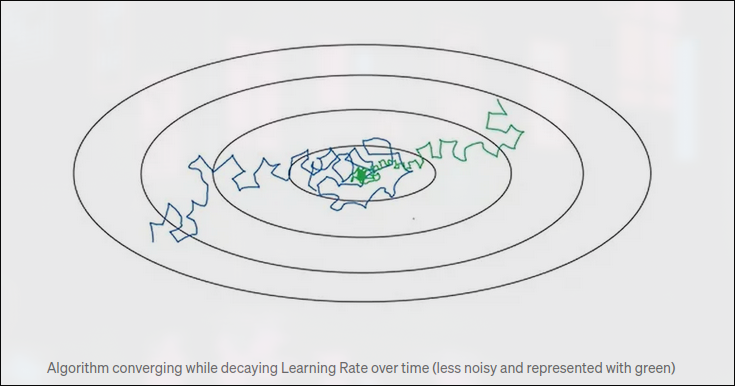
Learning rate decay is a technique for training modern neural networks. It starts training the network with a large learning rate and then slowly reducing/decaying it until local minima is obtained. It is empirically observed to help both optimization and generalization.
The preferred way to train a model to first overfit first train it as much data and as much model hyperparameters as possible, and then prevent overfitting using regularization techniques to prevent overfitting
- Data - our setup uses much less data (225 vs millions)
- learning rate warmup - start with a low learning rate and increase to the base LR
- learning rate decay - as model starts to converge, starts to lower LR
- Gradient clipping - prevents gradients from getting too big
Generally, in deep laerning if you can use a pretrained model from a large dataset on your own problem, it's often acheives great results with little data
Why use a pretrained model?
- Some times data is limited
- limiteed trainng resources
- get better results faster (maybe)
30 days is actually a smalll amount of time for large ML models, it is actually a small amount of time
# get pretrainedd wieghts for vit/b
pretrained_vit_weights = torchvision.models.ViT_B_16_Weights.DEFAULT #default = best available weights

#set up a vit model instance with pretrained weights
pretrained_vit = torchvision.models.vit_b_16(weights=pretrained_vit_weights).to(device)
pretrained_vit
VisionTransformer(
(conv_proj): Conv2d(3, 768, kernel_size=(16, 16), stride=(16, 16))
(encoder): Encoder(
(dropout): Dropout(p=0.0, inplace=False)
(layers): Sequential(
(encoder_layer_0): EncoderBlock(
(ln_1): LayerNorm((768,), eps=1e-06, elementwise_affine=True)
(self_attention): MultiheadAttention(
(out_proj): NonDynamicallyQuantizableLinear(in_features=768, out_features=768, bias=True)
)
(dropout): Dropout(p=0.0, inplace=False)
(ln_2): LayerNorm((768,), eps=1e-06, elementwise_affine=True)
(mlp): MLPBlock(
(0): Linear(in_features=768, out_features=3072, bias=True)
(1): GELU(approximate='none')
(2): Dropout(p=0.0, inplace=False)
(3): Linear(in_features=3072, out_features=768, bias=True)
(4): Dropout(p=0.0, inplace=False)
)
)
(encoder_layer_1): EncoderBlock(
(ln_1): LayerNorm((768,), eps=1e-06, elementwise_affine=True)
(self_attention): MultiheadAttention(
(out_proj): NonDynamicallyQuantizableLinear(in_features=768, out_features=768, bias=True)
)
...
)
(heads): Sequential(
(head): Linear(in_features=768, out_features=1000, bias=True)
)
)
for param in pretrained_vit.parameters():
    param.requires_grad = False

#update the classifier head
set_seeds()
pretrained_vit.heads = nn.Linear(in_features=768, out_features=len(class_names)).to(device) #also makes it trainable
============================================================================================================================================ Layer (type (var_name)) Input Shape Output Shape Param # Trainable ============================================================================================================================================ VisionTransformer (VisionTransformer) [1, 3, 224, 224] [1, 3] 768 Partial ├─Conv2d (conv_proj) [1, 3, 224, 224] [1, 768, 14, 14] (590,592) False ├─Encoder (encoder) [1, 197, 768] [1, 197, 768] 151,296 False │ └─Dropout (dropout) [1, 197, 768] [1, 197, 768] -- -- │ └─Sequential (layers) [1, 197, 768] [1, 197, 768] -- False │ │ └─EncoderBlock (encoder_layer_0) [1, 197, 768] [1, 197, 768] (7,087,872) False │ │ └─EncoderBlock (encoder_layer_1) [1, 197, 768] [1, 197, 768] (7,087,872) False │ │ └─EncoderBlock (encoder_layer_2) [1, 197, 768] [1, 197, 768] (7,087,872) False │ │ └─EncoderBlock (encoder_layer_3) [1, 197, 768] [1, 197, 768] (7,087,872) False │ │ └─EncoderBlock (encoder_layer_4) [1, 197, 768] [1, 197, 768] (7,087,872) False │ │ └─EncoderBlock (encoder_layer_5) [1, 197, 768] [1, 197, 768] (7,087,872) False │ │ └─EncoderBlock (encoder_layer_6) [1, 197, 768] [1, 197, 768] (7,087,872) False │ │ └─EncoderBlock (encoder_layer_7) [1, 197, 768] [1, 197, 768] (7,087,872) False │ │ └─EncoderBlock (encoder_layer_8) [1, 197, 768] [1, 197, 768] (7,087,872) False │ │ └─EncoderBlock (encoder_layer_9) [1, 197, 768] [1, 197, 768] (7,087,872) False │ │ └─EncoderBlock (encoder_layer_10) [1, 197, 768] [1, 197, 768] (7,087,872) False │ │ └─EncoderBlock (encoder_layer_11) [1, 197, 768] [1, 197, 768] (7,087,872) False │ └─LayerNorm (ln) [1, 197, 768] [1, 197, 768] (1,536) False ├─Linear (heads) [1, 768] [1, 3] 2,307 True ============================================================================================================================================ Total params: 85,800,963 Trainable params: 2,307 Non-trainable params: 85,798,656 Total mult-adds (M): 172.47 ============================================================================================================================================ Input size (MB): 0.60 Forward/backward pass size (MB): 104.09 Params size (MB): 229.20 Estimated Total Size (MB): 333.89 ============================================================================================================================================
When using a pretrained model we want to make sure our data is formatted same way the pretrained model was trained on
#get automatic transforms fromm pretrained VIT weights
vit_transforms = pretrained_vit_weights.transforms()
vit_transforms
ImageClassification(
crop_size=[224]
resize_size=[256]
mean=[0.485, 0.456, 0.406]
std=[0.229, 0.224, 0.225]
interpolation=InterpolationMode.BILINEAR
)
#setup dataloaders
from pytorch_modules.modules import data_preprocess
train_dataloader_pretrained, test_dataloader_pretrained, class_names = data_preprocess.create_dataloaders(train_dir=train_dir,
                                                                                                          test_dir=test_dir,
                                                                                                          transform=vit_transforms,
                                                                                                          batch_size=32, #could set a higher batch_size because using a pretrained model ( not many weightupdate needed) only have to update the MLP head weights as rest are untrainable
                                                                                                          )
train_dataloader_pretrained, test_dataloader_pretrained, class_names
(torch.utils.data.dataloader.DataLoader at 0x7fc9e0af7a50, torch.utils.data.dataloader.DataLoader at 0x7fc9e0c5be50, ['pizza', 'steak', 'sushi'])
 from pytorch_modules.modules import train_engine

#create optim and loss
optimizer = torch.optim.Adam(params=pretrained_vit.parameters(),
                             lr=1e-3)
loss_fn = torch.nn.CrossEntropyLoss()

#train the classifier head of the pretrained vit:
set_seeds()
pretrained_vit_results = train_engine.train(model=pretrained_vit,
                                            train_dataloader=train_dataloader_pretrained,
                                            test_dataloader=test_dataloader_pretrained,
                                            optimizer=optimizer,
                                            loss_fn=loss_fn,
                                            epochs=10,
                                            device=device,
                                            writer=None)
Epoch: 1 | train_loss: 0.7663 | train_acc: 0.7188 | test_loss: 0.5435 | test_acc: 0.8769 Epoch: 2 | train_loss: 0.3436 | train_acc: 0.9453 | test_loss: 0.3257 | test_acc: 0.8977 Epoch: 3 | train_loss: 0.2068 | train_acc: 0.9492 | test_loss: 0.2698 | test_acc: 0.9186 Epoch: 4 | train_loss: 0.1557 | train_acc: 0.9609 | test_loss: 0.2414 | test_acc: 0.9186 Epoch: 5 | train_loss: 0.1244 | train_acc: 0.9727 | test_loss: 0.2271 | test_acc: 0.8977 Epoch: 6 | train_loss: 0.1210 | train_acc: 0.9766 | test_loss: 0.2122 | test_acc: 0.9280 Epoch: 7 | train_loss: 0.0933 | train_acc: 0.9766 | test_loss: 0.2342 | test_acc: 0.8883 Epoch: 8 | train_loss: 0.0793 | train_acc: 0.9844 | test_loss: 0.2268 | test_acc: 0.9081 Epoch: 9 | train_loss: 0.1084 | train_acc: 0.9883 | test_loss: 0.2064 | test_acc: 0.9384 Epoch: 10 | train_loss: 0.0646 | train_acc: 0.9922 | test_loss: 0.1795 | test_acc: 0.9176
thats the power of transfer learning we managed to outperform our older model in no amount of time
now we've got a model that performs quite well, how about we save it to file then check it's filesize.
we want tot check the filesize because if we wanted to delpoy a model to website/mobile app, we may limitations o n the size of the model we can deploy.
Eg: smalller model way be required to due compute restrictions
#saving the model
from pytorch_modules.modules import utils
utils.save_model(model=pretrained_vit,
                 target_dir="models",
                 model_name="pretrained_vit_feature_extractor.pth")
[INFO] Saving model to: models/pretrained_vit_feature_extractor.pth
from pathlib import Path
#get the model size in bytes and then convert to megabytes
pretrained_vit_model_size = Path('models/pretrained_vit_feature_extractor.pth').stat().st_size // (1024**2)
print(f"Pretrained ViT model size: {pretrained_vit_model_size} MB")
Pretrained ViT model size: 327 MB
from helper_functions import pred_and_plot_image
pred_and_plot_image(model=pretrained_vit,
                    image_path='images/piza.jpg',
                    class_names=class_names)