Following the toy example we saw in the previous lesson, we shall now grow a decision tree for a more complex dataset. This lab covers all major areas of standard machine learning practice , from data acquisition to evaluation of results. We shall use scikit learn, pandas and graphviz libraries to conduct this analysis following the example of play tennis dataset.
You will be able to:
- Use pandas to prepare the data for the scikit-learn decision tree algorithm
- Train the classifier with a training dataset and evaluate performance using different measures
- Visualize the decision tree and interpret the visualization
In this lab we shall work with a popular dataset for classification called the "UCI Bank Note Authentication Dataset'. This Data were extracted from images that were taken from genuine and forged banknote-like specimens. The notes were first digitized, followed by a numerical transformation using DSP techniques. The final set of engineered features are all continuous in nature (visit the UCI link to learn about feature engineering in detail).
We have following attributes in the dataset.
- Variance of Wavelet Transformed image (continuous)
- Skewness of Wavelet Transformed image (continuous)
- Curtosis of Wavelet Transformed image (continuous)
- Entropy of image (continuous)
- Class (integer) - Target/Label
- Import necessary libraries as we saw in previous lesson
# Import necessary libraries

## Your code here - Read the file
"data_banknote_authentication.csv"as a pandas dataframe. Note that there is no header information in this dataset. - Assign column names 'Variance', 'Skewness', 'Curtosis', 'Entropy', 'Class' to dataset in the given order.
- View the basic statistics and shape of dataset.
- Check for frequency of positive and negative examples in the target variable
# Create Dataframe

## Your code here
# Describe the dataset
## Your code here .dataframe tbody tr th {
vertical-align: top;
}
.dataframe thead th {
text-align: right;
}
| Variance | Skewness | Curtosis | Entropy | Class | |
|---|---|---|---|---|---|
| count | 1372.000000 | 1372.000000 | 1372.000000 | 1372.000000 | 1372.000000 |
| mean | 0.433735 | 1.922353 | 1.397627 | -1.191657 | 0.444606 |
| std | 2.842763 | 5.869047 | 4.310030 | 2.101013 | 0.497103 |
| min | -7.042100 | -13.773100 | -5.286100 | -8.548200 | 0.000000 |
| 25% | -1.773000 | -1.708200 | -1.574975 | -2.413450 | 0.000000 |
| 50% | 0.496180 | 2.319650 | 0.616630 | -0.586650 | 0.000000 |
| 75% | 2.821475 | 6.814625 | 3.179250 | 0.394810 | 1.000000 |
| max | 6.824800 | 12.951600 | 17.927400 | 2.449500 | 1.000000 |
# Shape of dataset
## Your code here (1372, 5)
# Class frequency of target variable
## Your code here 0 762
1 610
Name: Class, dtype: int64
## Your Observations
So now we need to create our feature set X and labels y.
- Create X and y by selecting the appropriate columns from the dataset
- Create a 80/20 split on the dataset for training/testing. Use random_state=10 for reproducibility
# Create features and labels
## Your code here # Perform an 80/20 split
## Your code here - Create an instance of decision tree classifier with random_state=10 for reproducibility
- Fit the traiing data to the model
- USe the trained model to make predictions with test data
# Train a DT classifier
## Your code here DecisionTreeClassifier(class_weight=None, criterion='gini', max_depth=None,
max_features=None, max_leaf_nodes=None,
min_impurity_decrease=0.0, min_impurity_split=None,
min_samples_leaf=1, min_samples_split=2,
min_weight_fraction_leaf=0.0, presort=False, random_state=10,
splitter='best')
# Make predictions for test data
## Your code here We can now use different evaluation measures to check the predictive performance of the classifier.
- Check the accuracy , AUC and create a confusion matrix
- Interpret the results
# Calculate Accuracy , AUC and Confusion matrix
## Your code here Accuracy is :97.81818181818181
AUC is :0.98
Confusion Matrix
----------------
.dataframe tbody tr th {
    vertical-align: top;
}

.dataframe thead th {
    text-align: right;
}
| Predicted | 0 | 1 | All |
|---|---|---|---|
| True | |||
| 0 | 149 | 3 | 152 |
| 1 | 3 | 120 | 123 |
| All | 152 | 123 | 275 |
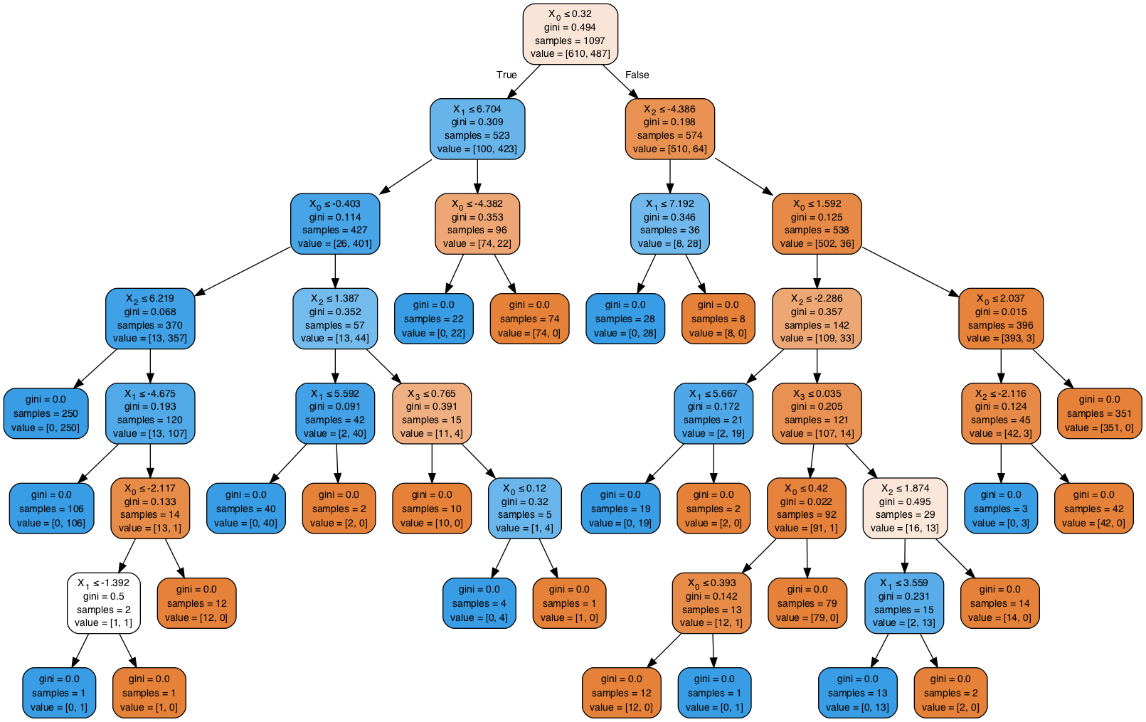
# Your observations here - Use graphviz to visualize the tree
- Interpret the results
# Visualize the tree trained from complete dataset

## Your code here
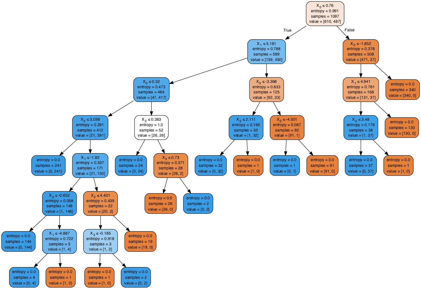
## Your observations hereSO in the above example, we used all default settings for decision tree classifier. The default impurity crietrion in scikit learn is the Gini impurity. We can change it back to entropy by passing in criterion='entropy' argument to the classifier in the training phase.
- Repeat the above tasks for training, evaluation and visualization using Entropy measure. (
- Compare and interpret the results
## Your code here
Accuracy is :99.63636363636364

AUC is :1.0

Confusion Matrix
----------------
Predicted    0    1  All
True
0          151    1  152
1            0  123  123
All        151  124  275
# Your observations here

# With entropy we see a much lower accuracy and AUC than earlier
# Only one false positive value , leading to accuracy of 99%
# The tree shape changes considerably with change in impurity criteria - We discussed earlier that decision trees are very sensitive towards outliers. Try to identify and remove/fix any possible outliers in the dataset.
- Check the distributions of the data. Is there any room for normalization/scaling of data ? Apply these techiques and see if it improves upon accuracy score.
In this lesson, we looked at growing a decision tree for banknote authentication dataset which is composed of extracted continuous features from photographic data. We looked at different stages of the experiment including data acquisition, training, prediction and evaluation. We also looked at growing trees using entropy vs. gini impurity criteria. In following lessons, we shall look at some more such pre-train tuning techniques for ensuring an optimal classifier for learning and prediction.

