spolivin / rearden

Library of useful data structures for data preprocessing (spacial/time-series), vizualizations and grid search

Rearden

Rearden is a Python package designed for usage inside Jupyter Notebooks that provides a faster and more convenient way of carrying out data science and getting insights from machine learning algorithms. Making use of the functionality of the most popular libraries for data analysis (pandas, numpy, statsmodels), data visualization (matplotlib, seaborn) and grid search (scikit-learn), it enables reaching the conclusions about the data in a quicker and clearer manner.

---

Modules and API

The package is designed to aid data scientists in quickly getting insights about the data during the following stages of data analysis/machine learning:

• Data preprocessing
• Data visualization
• Time-series analysis
• Grid search

Hence, the data structures which make up the Rearden package have been logically divided into the following Python modules (module decorators.py serves as an auxiliary file supplying the decorators for some data structures includes in the other modules):

• preprocessings.py
• vizualizations.py
• time_series.py
• grid_search.py
• metrics.py

Data preprocessing

Functions included in preprocessings.py are basically programmed to help with missing values and data preparation for machine learning algorithms (e.g. data split into sets). For instance, currently the following functions and classes are included in the module:

Name	Kind	Description
DataSplitter	class	Data split into sets depending on target name and sets proportions
identify_missing_values	function	Display of the number and share of missing values

The module and the associated functions can be called like so:

from rearden.preprocessings import DataSplitter

Splitting data

For instance, if we have a pandas DataFrame which includes both features and target, we can easily separate them into distinct entities and at the same time split them into training/test sets:

from rearden.preprocessings import DataSplitter

splitter = DataSplitter(set_shares=(0.75, 0.25), random_seed=1)

(
features_train,
target_train,
features_test,
target_test
) = splitter.split_data(data=some_dataframe, target="target_name")

Likewise, if we need to split the DataFrame into training/validation/test sets:

splitter = DataSplitter(set_shares=(0.6, 0.2, 0.2), random_seed=1)

(
features_train,
target_train,
features_valid,
target_valid,
features_test,
target_test
) = splitter.split_data(data=some_dataframe, target="target_name")

Afterwards, it is possible to check the splits via a special subset_info_ attribute:

splitter.subset_info_

We will get the following table:

	obs_num	set_shares
train	5,454	0.6
valid	1,818	0.2
test	1,819	0.2

In case we have intended to split the data only into training and test sets, the DataFrame contained in subset_info_ attribute becomes as follows:

	obs_num	set_shares
train	6,818	0.75
test	2,273	0.25

All data subsets obtained as a result of a DataFrame split are contained in the according attributes of the class and can be used at any time:

features_train = splitter.features_train_
features_valid = splitter.features_valid_
features_test = splitter.features_test_

target_train = splitter.target_train_
target_valid = splitter.target_valid_
target_test = splitter.target_test_

Thanks to decorators provided in decorators.py, the potential errors which can be made during the instantiation of the class object or during the data split can be caught faster. For instance, check_proportions decorator from DataSplitterDecorators class will check the correctness of set shares specification in set_shares attribute when defining an object. Decorator check_dimensions will make sure that we specify two or three values in set_shares attribute. Lastly, check_split will catch the user's mistake of accessing subset_info_ attribute before data split has occurred.

Missing values calculation

Using a useful identify_missing_values function, it is possible to quickly calculate the number and share of missing values in a DataFrame. Furthermore, it also outputs the data type of a column where missing values have been found. For instance:

identify_missing_values(data=some_dataframe)

The resulting DataFrame looks as follows:

	dtype	missing_count	missing_fraction
col1	float64	400	0.8444
col3	object	19	0.4512
col19	object	4	0.0313

In the case that no missing values have been detected, the function will not return anything.

Data visualization

Enhanced data vizualizations tools are located in vizualizations.py module. The functions here are as follows:

Name	Kind	Description
plot_model_comparison	function	Visualization of ML models performances based on their names and scores
plot_corr_heatmap	function	Plotting correlation matrix heatmap in one go
plot_class_structure	function	Plotting the shares of different classes for a target vector in classification problems

Models performance comparison

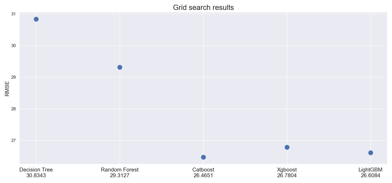
Using plot_model_comparison function, it is very easy to conveniently showcase how models perform according to some metric. One would just run:

import seaborn as sns

from rearden.vizualizations import plot_model_comparison

sns.set_theme()

models_performance = [
    ("Decision Tree", 30.8343),
    ("Random Forest", 29.3127),
    ("Catboost", 26.4651),
    ("Xgboost", 26.7804),
    ("LightGBM", 26.6084),
]

plot_model_comparison(
    results=models_performance,
    metric_name="RMSE",
    title_name="Grid search results",
    save_fig=True,
)

The result is the following figure which is automatically saved in the newly created images directory upon specifying save_fig=True (setting this parameter to True automatically activates rearden.vizualizations.save_plot_in_dir function that creates images/ directory and saves the image there):

Correlation matrix heatmap

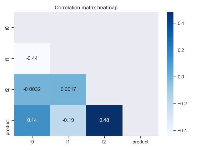
It is possible to quickly plot the heatmap of the correlation matrix for the data using plot_corr_heatmap function. Here is how we would do that:

import pandas as pd
import seaborn as sns

from rearden.vizualizations import plot_corr_heatmap

sns.set_theme()

test_data = pd.read_csv("datasets/test_data.csv")

plot_corr_heatmap(
    data=test_data,
    heatmap_coloring="Blues",
    annotation=True,
    lower_triangle=True,
    save_fig=True,
)

The code above results in the following plot:

Plotting the class structure

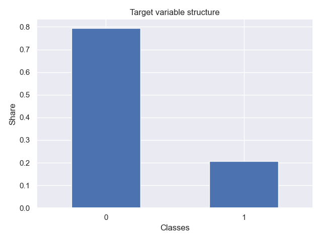
The function plot_class_structure enables quickly making inquiries into the balancedness/unbalancedness of the target variable:

from rearden.vizualizations import plot_class_structure

plot_class_structure(
    target_var=target_train,
    xlabel_name="Classes",
    ylabel_name="Share",
    title_name="Target variable structure",
    save_fig=True,
)

The resulting plot looks, for instance, as follows:

Time-series analysis

Tools for time-series analysis from time_series.py are pretty straightforward:

Name	Kind	Description
TimeSeriesFeaturesExtractor	class	Extraction of time variables from a one-dimensional time-series depending on lag and rolling mean order values
TimeSeriesSplitter	class	Time-series data split into sets with the same functionality as DataSplitter
TimeSeriesPlotter	class	Plotting the original time-series or a decomposed one

One can, for example, want to firstly look at the graph via TimeSeriesPlotter, recover time variables from time-series by TimeSeriesFeaturesExtractor and then divide the data into sets with TimeSeriesSplitter.

Time-series plot and its decomposition

TimeSeriesPlotter class provides two additional ways we could plot a time-series:

• Plain time-series (plot_time_series method)
• Decomposed time-series: trend, seasonality, residual (plot_decomposed method)

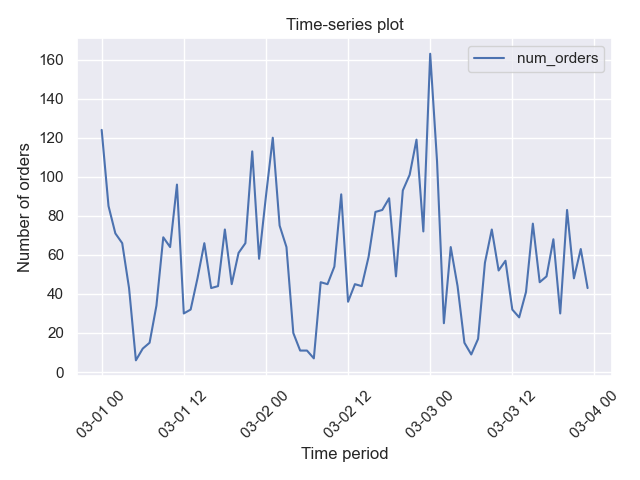
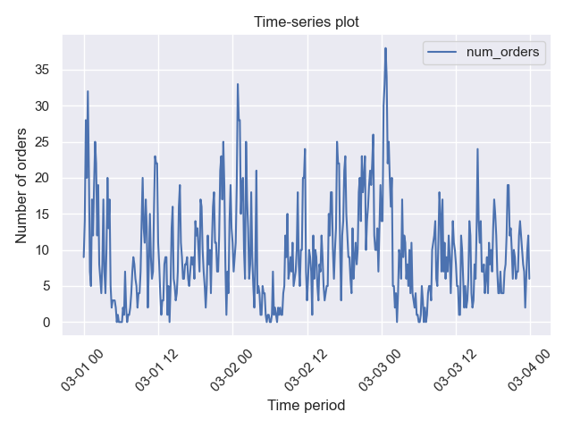
For example, we can plot the resampled time-series data (with 1 hour periodicity by default):

import pandas as pd
import seaborn as sns

from rearden.time_series import TimeSeriesPlotter

sns.set_theme()

ts_data_test = pd.read_csv("datasets/ts_data_test.csv", parse_dates=[0], index_col=[0])

ts_plotter = TimeSeriesPlotter()

plotter.plot_time_series(
    data=taxi_data,
    resample=True,
    period=("2018-03-01", "2018-03-03"),
    ylabel_name="Number of orders",
    title_name="Time-series plot",
    save_fig=True,
)

In this case we plot the evolution of the number of orders against time. We obtain the following plot:

If we want to plot the time-series for the same period of time without resampling, then we just set resample=False:

plotter.plot_time_series(
    data=taxi_data,
    resample=False,
    period=("2018-03-01", "2018-03-03"),
    ylabel_name="Number of orders",
    title_name="Time-series plot",
    save_fig=True,
)

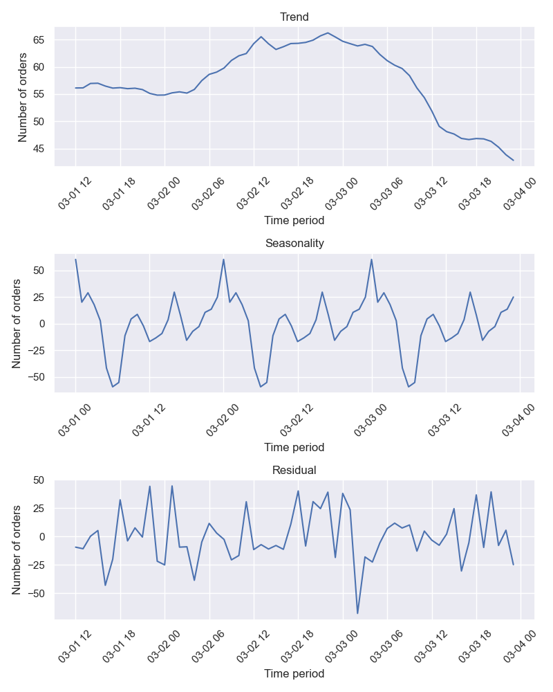
We could also decompose this time series which in this case should be resampled in any case (applied by default):

plotter.plot_decomposed(
    data=taxi_data,
    period=("2018-03-01", "2018-03-03"),
    ylabel_name="Number of orders",
    save_fig=True,
)

The result is as follows:

Creating time features

Given the one-dimensional time-series data, it is actually possible to retrieve time variables from it: quarter, month, day or month. Additionally, we can also add lags as well as rolling mean of different orders. It can be done using TimeSeriesFeaturesExtractor:

from rearden.time_series import TimeSeriesFeaturesExtractor as TSFE

features_extractor = TSFE(col_name="num_orders")
features_extractor.get_params() # {'col_name': 'num_orders', 'max_lag': 1, 'rolling_mean_order': 1}

Hence, we can choose the column with the time-series as well as which maximum order of lag and rolling mean we want to use when generating new features. For instance, if we decide to use the default parameter values, we can easily configure the class and then use it on the data:

import pandas as pd

ts_data_test = pd.read_csv("datasets/ts_data_test.csv", parse_dates=[0], index_col=[0])
ts_data_test = ts_data_test.resample("1H").sum()

ts_dataset = features_extractor.fit_transform(ts_data_test)

The above code will add quarter, month, day and hour variables to the DataFrame as well as a column with rolling mean and the lag columns according to max_lag and rolling_mean_order attribute values.

Grid search

In grid_search.py module, RandomizedSearchCV base class from sklearn.model_selection was used, which has been wrapped with two additional classes with some additional methods, custom defaults and other functionality:

Name	Kind	Description
RandomizedHyperoptRegression	class	Wrapper for RandomizedSearchCV with functionality to quickly compute regression metrics and conveniently display tuning process
RandomizedHyperoptClassification	class	Wrapper for RandomizedSearchCV with functionality to quickly compute classification metrics, conveniently display tuning process and fastly plot confusion matrix
SimpleHyperparamsOptimizer	class	Custom class that implements a simple grid search algorithm without cross-validation

The module also includes one custom SimpleHyperparamsOptimier class written from scratch that enables quickly running a grid search when, for instance, we need to optimize the hyperparameters of the model on one distinct validation set.

Hyperparameter tuning

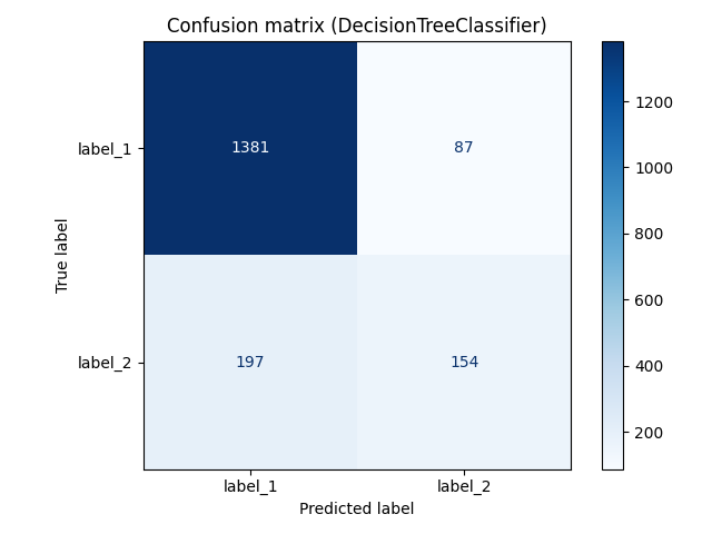
We can use RandomizedHyperoptClassification or RandomizedHyperoptRegression wrappers for quickly making conclusions about the results of the grid search. For instance, let's imagine that we have managed to split the data into features_train and features_test as well as target_train and target_test. We can now run the grid search algorithms and immediately get the plot of the confusion matrix:

from sklearn.tree import DecisionTreeClassifier

from rearden.grid_search import RandomizedHyperoptClassification as RHC

dtc_model = DecisionTreeClassifier(random_state=12345)
param_grid_dtc = {"max_depth": np.arange(2, 12)}

dtc_grid_search = RHC(
    estimator=dtc_model,
    param_distributions=param_grid_dtc,
    train_dataset=(features_train, target_train),
    eval_dataset=(features_test, target_test),
    random_state=12345,
    cv=5,
    n_iter=5,
    scoring="f1",
    n_jobs=None,
    return_train_score=True,
)
dtc_grid_search.train_crossvalidate()

After the completing grid search, the method train_crossvalidate will notify us of the completion:

Grid search for DecisionTreeClassifier completed.
Time elapsed: 0.6 s

Tuning process display

We can then get a convenient representation of the tuning progress by using display_tuning_process method:

dtc_grid_search.display_tuning_process()

	max_depth	mean_test_score	mean_train_score
0	2	0.4970	0.5065
1	9	0.5448	0.7347
2	5	0.5059	0.5379
3	11	0.5402	0.8257
4	8	0.5432	0.6869

Since this class inherits from sklearn.model_selection.RandomizedSearchCV, it also has access to usual best_estimator_, best_score_, best_params_ attributes.

Metrics computation

Thanks to the additional eval_dataset attribute, the resulting plot is already a confusion matrix for the best model after cross-validation which has been used for making predictions on the test data:

It is also possible to compute all classification metrics using classif_stats_ attribute that just outputs the result of applying sklearn.metrics.classification_report to data contained in eval_dataset attribute.

Other functionality of the wrappers for classification and regression can be consulted in the grid_search.py module.

Custom grid search without CV

A simple grid search algorithm has been implemented in SimpleHyperparamsOptimizer class. The usage is similar to sklearn grid search but without crossvalidation:

from sklearn.metrics import mean_squared_error

from rearden.grid_search import SimpleHyperparamsOptimizer as SHO

decision_tree_model = DecisionTreeRegressor(random_state=12345)
decision_tree_params_grid = {"max_depth": np.arange(1, 5)}

sho_search = SHO(
    model=decision_tree_model,
    param_grid=decision_tree_params_grid,
    train_dataset=(features_train, target_train),
    eval_dataset=(features_test, target_test),
    scoring_function=mean_squared_error,
    display_search=True,
    higher_better=False,
)
sho_search.train()

Since we set display_search=True, we will see the following grid search progress information:

{'max_depth': 1}: mean_squared_error=(train=1087.6845, valid=5115.3861)
{'max_depth': 2}: mean_squared_error=(train=915.5997, valid=4915.6283)
{'max_depth': 3}: mean_squared_error=(train=772.2890, valid=3686.3358)
{'max_depth': 4}: mean_squared_error=(train=696.7085, valid=3352.8290)

We can use the class attribute after calling train to obtain the best model settings and results:

sho_search.best_config_ # {'max_depth': 4}
sho_search.best_result_ # 3352.8289830072163

Installation

Package dependencies

Rearden library requires the following dependencies:

Package	Version
Matplotlib	>= 3.3.4
Pandas	>= 1.2.4
NumPy	>= 1.24.3
Scikit-learn	>= 1.1.3
Seaborn	>= 0.11.1
Statsmodels	>= 0.13.2

NOTE: The package currently requires Python 3.9 or higher.

Installation using pip

The package is available on PyPI Index and can be easily installed using pip:

pip install rearden

The dependencies are automatically downloaded when executing the above command or can be installed manually using (after cloning the repo):

pip install -r requirements.txt

Building the package

Thanks to the build system requirements and other metadata specified in pyproject.toml it is easy to build and install the package. Firstly, clone the repository:

git clone https://github.com/spolivin/rearden.git

cd rearden

Then, one can simply run the following:

pip install -e .

Automatic code style checks

Installation of pre-commit

Before pushing the changed code to the remote Github repository, the code undergoes numerous checks conducted with the help of pre-commit hooks specified in .pre-commit-config.yaml. Before making use of this feature, it is important to first download pre-commit package to the system:

pip install pre-commit

or if rearden package has already been installed (pre-commit is installed together with the linters):

pip install rearden[linters]

Afterwards, in the git-repository run the following command for installation:

pre-commit install

Now, the pre-commit hooks can be easily used for verifying the code style.

Pre-commit hooks

After running git commit -m "<Commit message>" in the terminal, the file to be committed goes through a few checks before being enabled to be committed. As specified in .pre-commit-config.yaml, the following hooks are used:

Hooks	Version
Pre-commit-hooks	4.3.0
Pyupgrade	3.10.1
Autoflake	2.1.1
Isort	5.12.0
Black	23.3.0
Flake8	6.0.0
Codespell	2.2.4

NOTE: Check .pre-commit-config.yaml for more information about the repos and hooks used.