The Discrete Spectral Transformation (“DST”) has been developed as an alternative to the Discrete Fourier Transformation (“DFT”) and it's fast variant, the Fast Fourier Transformation (“FFT”).
While the FFT works very well and fast when determining the spectrum of a signal now and then, it does not all work well when applied on a sample-by-sample level:
- Given an algorithmic performance of O (n*log(n)), where n is the window size of the FFT, computating the FFT for a series of m adjacent samples in a signal results in O (m*n*log(n)).
- The Fourier Transformation is designed to be applied on the complete signal, starting from indefinite past and reaching into indefinite future: the Fourier integral integrates from t=-∞ to t=+∞, and the Fourier series assumes the signal is periodic. Since in real-world applications, only a limited time range of a technical signal is available, a window function is used to mask a region of interest in the signal, and this region is used for a periodic continuation of the signal. This is fine, if the window is large and the spectrum does not change quickly, but it will lead to major inaccuracy otherwise. Even worse, since the signal is periodically continuated, at the point of continuation, the function will usually be non-steady, thus leading to high peaks in the resulting spectrum from the DFT or FFT, just for the fact that the original signal was tweaked by continuation. Therefore, the window function is usually combined with a Gausian filter that fades out the signal towards the continuation point, to avoid these peaks. This way, however, the resulting spectrum becomes even more imprecise and exhibits even slower response to quick changes in the spectrum. While this objective may sound strange, there is a convincing example. Imagine a signal consisting purely of a constant sine wave that, after a long time, is suddenly turned off, thus leaving perfect silence. When the sine wave stops, the spectrum should also fade out and approximate to perfect silence. However, the spectrum of a Fourier transform is not a function over time: it does not contain time as parameter, in contrast to the signal. That is, it does not matter if the sine wave has already stopped or not – the spectrum is always the same.
In contrast, the DST is designed to be applied on a sample-by-sample level. Rather than re-computing the spectrum from scratch for each sample, it re-uses the result from the previous calculation of the spectrum, and just considers, how the next samples changes the spectrum. That is, for each new sample, the spectrum is updated to include the contribution of that sample to the current spectrum. Also, the spectrum fades out in a way such that the contribution of samples seen long ago continously decreases.
The DST beats the DFT / FFT in terms of computational complexity, if a sample-by-sample series of spectrum frames is to be computed. However, the FFT beats the DST for the computation of a single spectrum frame.
For a single determination of the spectrum over m=n samples, the FFT with window size n takes O (n*log(n)), while the DST takes O (m*n)=O (n²) for m samples and n spectrum lines. That is, for determining once the spectrum over a limited range of a single, FFT is faster than DST.
However, for a series of spectrum analyses on a sample-by-sample basis over m samples, FFT takes O (m*n* log (n)), while DST only requires O (m*n).
DFT and DST can be parallelized by computing each spectral line by a completely separate processor, just sharing the same input signal. In contrast, the FFT uses a matrix multiplication (in order to reduce the number of multiplications) such that parallelization is limited. The butterfly step in the course of an FFT computation can not be fully parallelized due to the data dependencies across the spectral lines.
When computing all spectral lines independently from each other on a separate processor, the DST performs in O(1) for updating the spectral line when processing the next sample, assuming the number of available processors grows with the number of spectral line to be processed. The DST takes O(m) for the same task, assuming a window with m samples.
There are various approaches to parallize FFT, but as far as to my knowledge, all of them have at least O(log n) complexity.
DST as well as DFT and FFT assume discrete time and thus will have by design DFT and FFT use a window function and typcially a Gaussian filter, thus resulting in imprecise calculation of the spectrum and slow response to quick changes in the spectrum. The DST, however, gives more precise results and has much higher response to quick changes in the spectrum.
In my original conference presentation [Reuter:2009a], I stated that for the reverse transformation of the DST, while the mathematical foundation is clear, I still have no practical algorithm. In fact, at that time I already almost had a working algorithm; it turned out there just was a subtle bug in the numeric processing of complex numbers. Actually, the reverse transformation mostly boils down to summing up all values of the spectral lines of the transformed signal. This characteristics is what you really should expect from a transformation that deserves the attribute “spectral” in its name. For implementation details, just have a look at method 'getReconstructedSample()' in class 'DSTSlidingWindow' to see how simple it works.
The current DST implementation still has problems with numerical stability. While for a limited number of subsequent samples the reverse transformation works fine, when reverting a large number of successive samples, spectral lines have a tendency to produce small oscillations that contribute to a distorted reconstruction of the signal. I am still working on alleviating this deficiency.
The DST uses a coupling constant named μ0, a dimensionless quantity that determines how much influence the next sample has and how fast the contribution of past samples fades out. One can think of a strong correlation between the coupling constant and the turnover frequency τ in a low pass filter, especially if implemented as a discrete infinite impulse response filter.
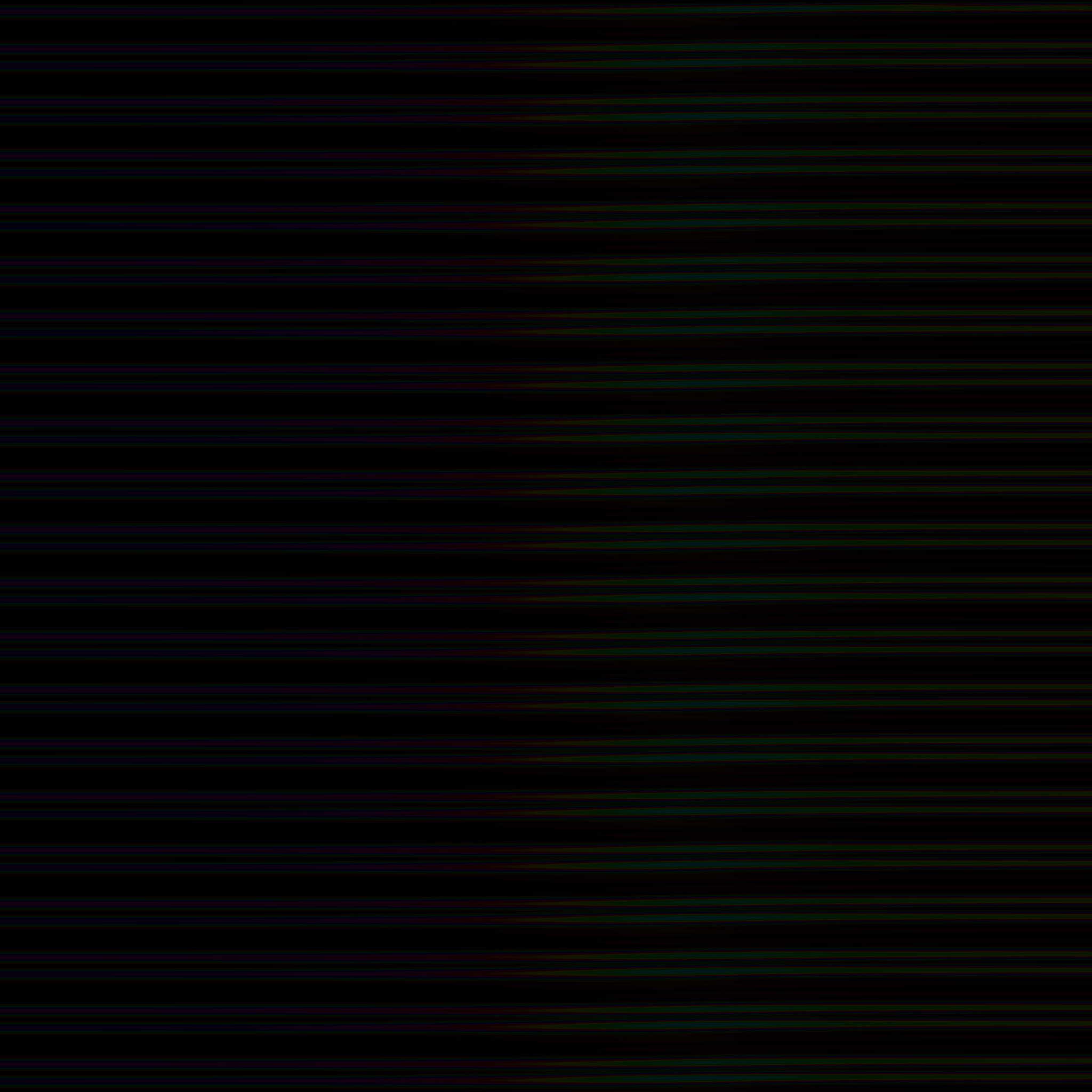
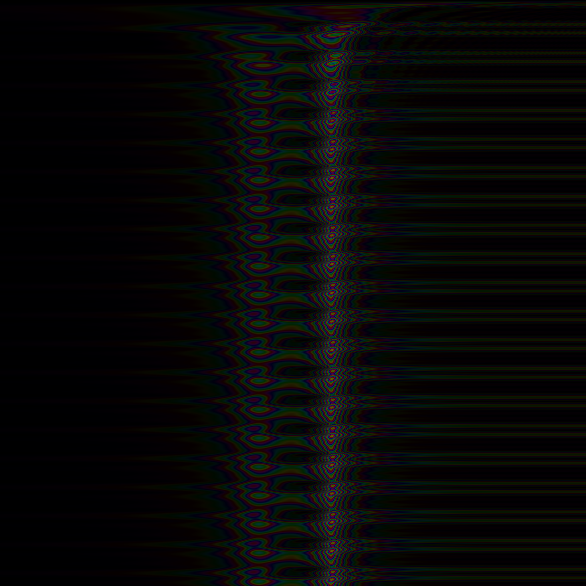
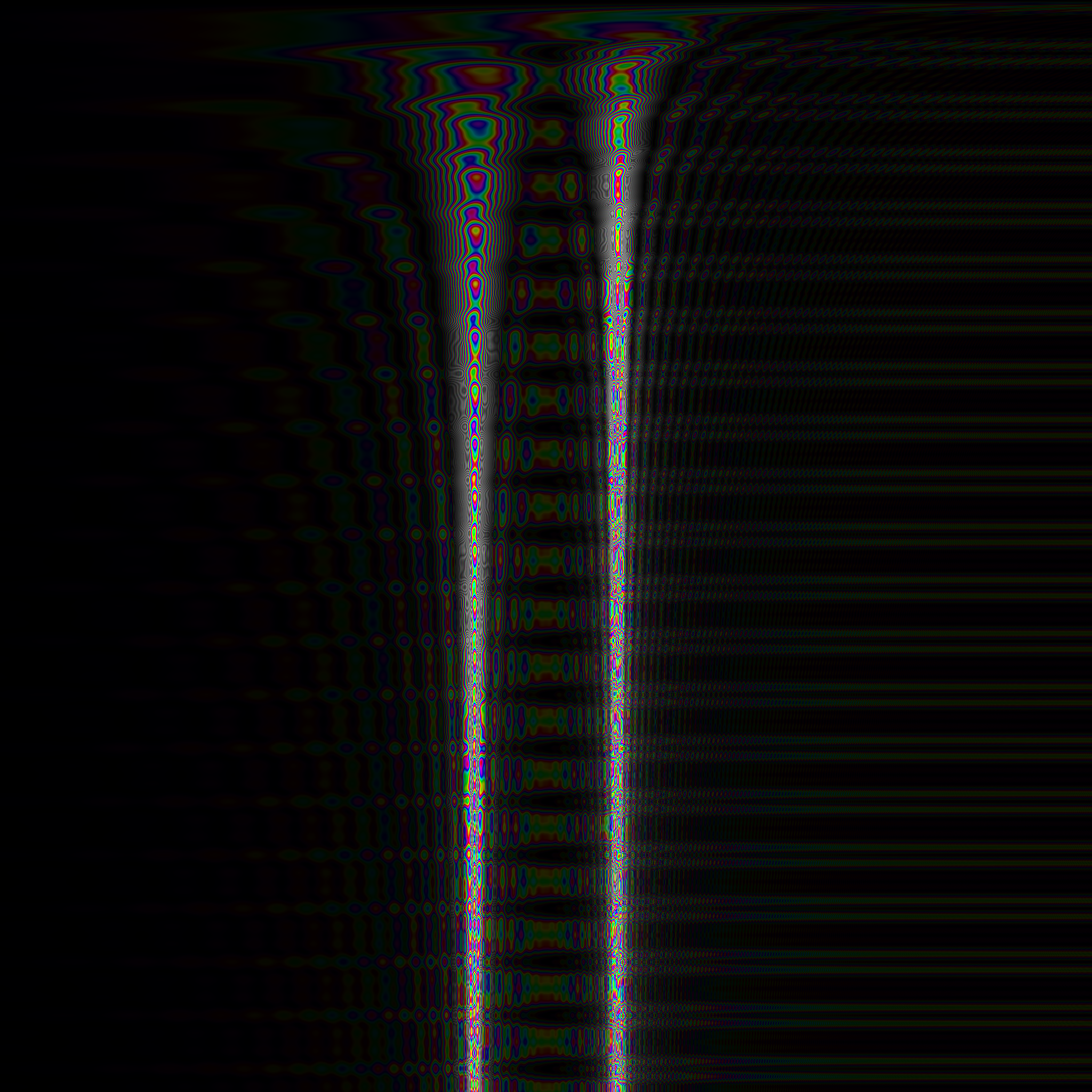
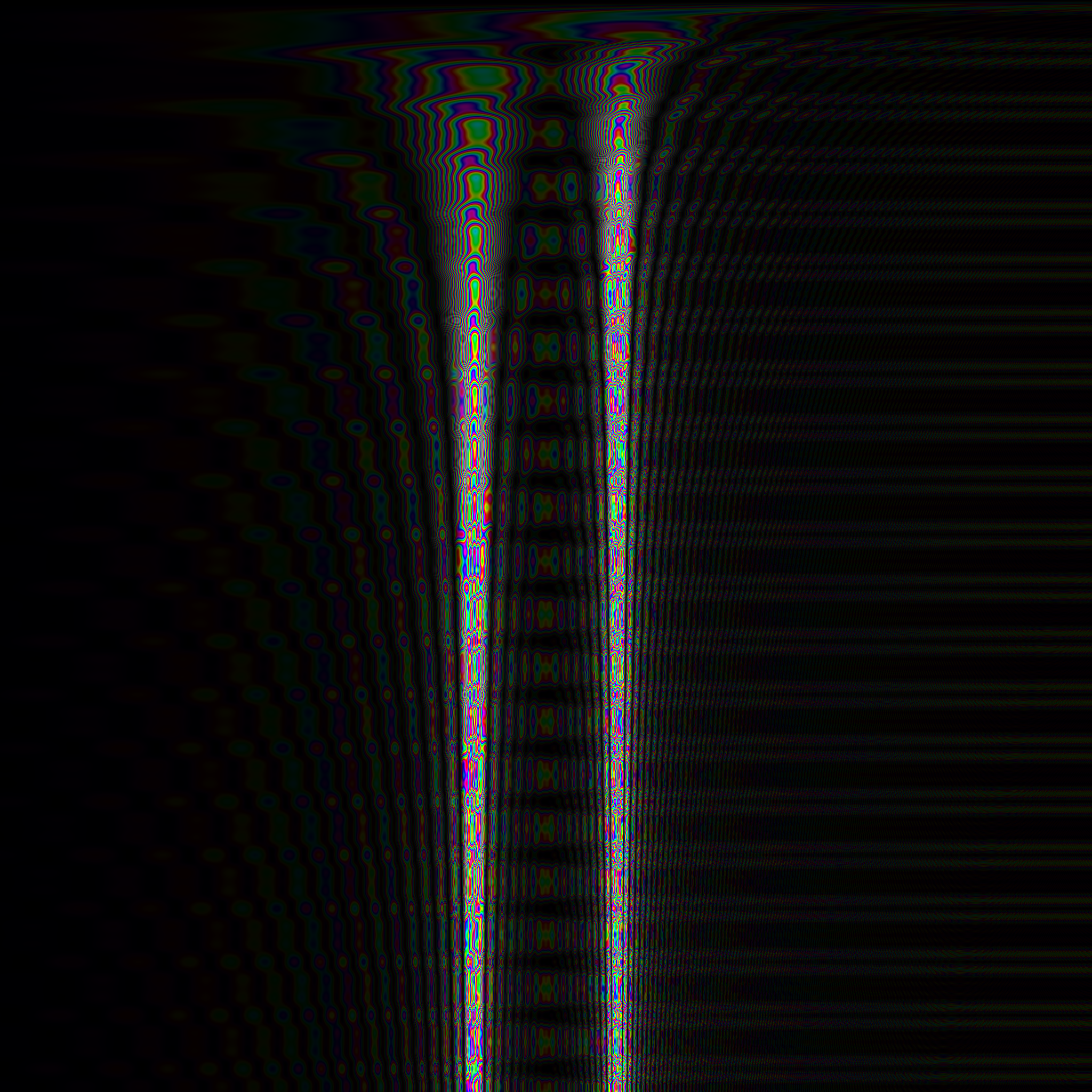
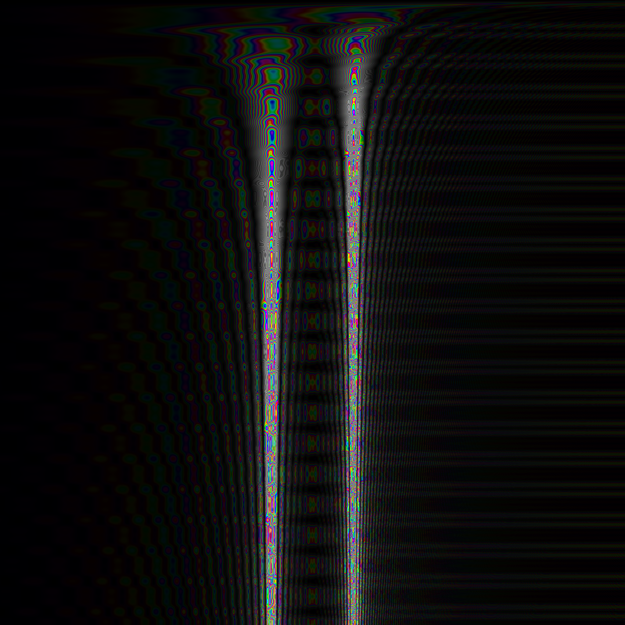
The following series of spectrum views depicts the behavior of the DST for varying values of the coupling constant. The diagrams show the spectrum with the time axis from top to down, and the frequency axis from left to right. The value of μ0 must be less than 1 for the integral of the DST transformation to converge. The higher the value, the greater the influence of past samples is retained, but also the slower the DST reacts to quick changes in the spectrum, as the following figures show for several values of μ0.
Fig. 1a: μ0 = 0.9
Fig. 1b: μ0 = 0.99
Fig. 1c: μ0 = 0.999
Fig. 1d: μ0 = 0.9999
Fig. 1e: μ0 = 0.99999
Fig. 1: DST Convergence for Combined 440Hz+880Hz Sine Waves @ 44.1kHz Sample Frequency
The figures suggest that the value of the coupling constant should be greater than 0.99 in order to retrieve good accuracy, but values greater than 0.999 do not add much more to it, but degrade responsiveness in the case of a quickly changing spectrum. Hence, a good trade-off between accuracy and responsiveness (this is a kind of uncertainty relation!) is a value inbetween, e.g. the value 1-α with α := 1 - 150√(1/3), where 150√(x) denotes the 150th root of x, i.e. 150√(x) := exp (1 / 150 * log (x)). Thus, the expression results in α ≈ 0.007297326 or μ0 ≈ 0.992702673.
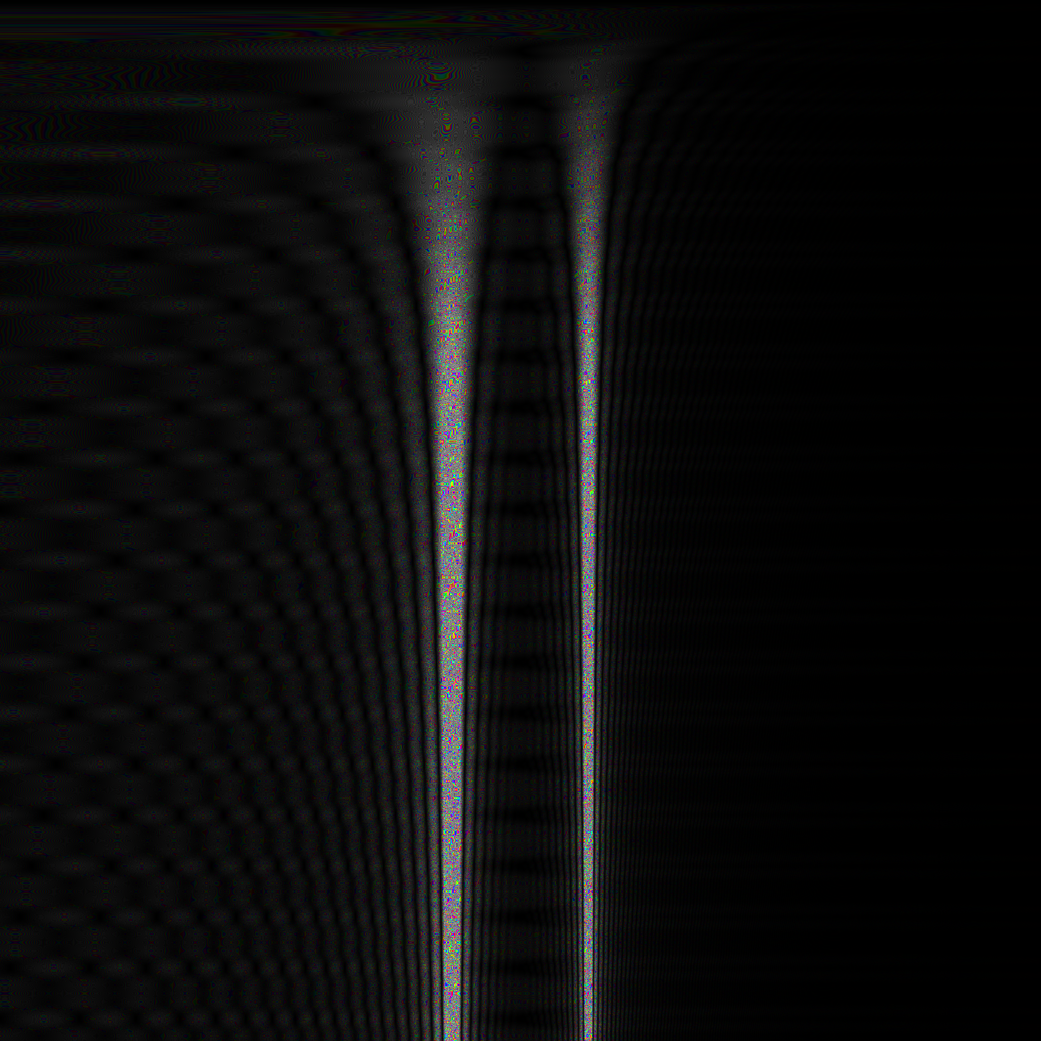
For better comparison, the library not only features the DST implementation, but also comprehends a sliding window implementation of a DFT. This DFT implementation keeps track of all sample values in the window with a ring buffer: each time a new sample is added to the window, the oldest one is kicked off. No Gaussian or other filter is applied. Note that this DFT implementation is feasible only for small window sizes due to the ring buffer. The DST does not need such a ring buffer, since instead, old samples are faded out. Since in this DFT implementation old samples are not faded out until they fall off from the window, new incoming samples affect the overall spectrum of the DFT much less. As a consequence, the DFT responses much more slowly to quick changes in the spectrum. For steady signals however, this DFT implementation works almost equally well compared to the DST, while still having the overhead of keeping track of all samples in the window.
Fig. 2: Sliding Window DFT
Note that — while so far mostly applied on accoustics — the DST may be applied to any field in physics where decomposition of a signal into sinoidal waves is desired.
Also note that the DST has some remarkable differences compared to the DFT:
-
The DFT's symmetry of cause and effect is mainly due to the symmetric bounds of the integral of the Fourier transform or the signal periodicity for a Fourier series. In contrast, the integral of the DST is bound to (-∞,0], thus keeping direction of causality.
-
The Fourier transform abstracts from the signal's t parameter, such that it does not occur any more in the transformed signal. In contrast, the DST preserves the t parameter, thus keeping an additional variable in the frequency space. This additional variable can be viewed as a hidden variable (in the sense as some authors assume for Quantum mechanics) of the Fourier transform, explicitly made accessible via the DST: For any point t1 in time, the DST for that point can be computed solely from the DST for any earlier point t0 in time and the signal between these two points t0 and t1, as shown in Eqn. 24 in the paper in Sect. 4.3 “Discretization” [Reuter:2009a]. That is, the DST for t0 holds all necessary information from the complete history before t0 that is required for computing the DST of some later point t1.
The following ideas in this section are random number and expression patterns that I recognized while working on the overall concepts.
DISCLAIMER: Please do not take these ideas as necessarily real physical facts, but just as inspiring ideas for working out future concepts. Having that said, here we go.
Remember that the non-negative parameter μ0 in our transformation serves as a constant for coupling over time, i.e. how fast the effect of the signal onto the spectrum decays over time. For the transformation's integral to converge, this constant requires to have a value of less than 1. In the course of this loose discussion however, just forget for a moment about this requirement. Actually, we are not going to compute the transformation here, hence we do not need the integral to converge.
In physics there is actually something like a coupling constant: the fine structure constant α ≈ 7.297353e-3. Let's take the value of 1 / α ≈ 137.036 as value for μ0, even though it is not less than 1, but much greater than 1. In our transformation, the parameter appears as part of exponent of the natural e function, i.e. we consider the expression exp(1 / α).
Next, in the paper, we reason about discretization of the transformation. In physics, is there a discretization in terms of space? In some sense, there probably is: The Planck length lp ≈ 1.616e-35m. Let us take this value as basic unit, i.e. as a factor multiplied with what to come next.
Finally, remember that our transformation is scaled with a factor equal to the constant value that appears in the exponent of the e function. Let's do this here as well, i.e. scale the expression by the factor (1 / α).
So, altogether, in terms of α, we get the function
f(α) := lp * (1 / α) * exp(1 / α)
which evaluates to
f(α) ≈ 7.231e26m.
Maybe think of a wave with an extremely low frequence, maybe just as low that is spreads out just making up a single, huge period that covers all of the universe that we can recognize. The minimum extent of the universe is that of the observable universe and is said to be around 93 billions (93 * 109) of light-years [Wikimedia:2019a]. Note that physicists believe in something called dark matter that is thought to make up maybe up to 85% of all matter, thus making the real size of the universe much bigger, without being able to quantify that size. For the purpose of our discussion, let's consider just the observable part of the universe, thus assuming an extent of roughly 93 light-years.
With 1 light-year = 1ca (with letter c denoting speed of light and letter a denoting a year), we get an extent d of
d ≈ 93e9ca ≈ 93e9 * 3e8 m/s * 365.25 * 24 * 60 * 60 s ≈ 8.804e26m
Well, d ≈ 8.804e26m and f(α) ≈ 7.231e26m are pretty close, aren't they? They are off not much more than 20% from each other, while spanning a range of 61 decades from lp to d.
Hence, let us assume these two numbers are actually identical, and the difference only results from measurement tolerance.
Next, we assume an almost linear expansion of the universe, according to the Lambda-CDM model [Wikimedia:2019b], [Wikimedia:2017] during its age of roughly 13.8e9 years. In fact, current theories assume that the very early universe expanded more quickly, and then expansion slowed down, but nowadays expansion tends to slowly speed up again. We assume these limited abberation from linear expansion to have only little effect on our computations, such that for a first approximation, they can be neglected.
Finally, we do not try to explicitly consider relativistic effects in our computations, since we think that they are either neglectible or already implicitly considered by using physical constants that others already have computed.
Most of these assumptions are very audacious and may turn out to be completely wrong. Nevertheless, given that all of these assumptions turn out to be true, we can compute an approximation of the drift of the the fine structure constant over time:
In case all of our assumptions will hold true, we predict that the fine structure constant should currently decrease by a value of roughly 3.83e-15 per year.
The computation is elaborated in the Java files
SolveExpEqDouble.java and SolveExpEqBigDecimal.java, respectively.
SolveExpEqDouble is an implementation with 64 bit floating point
arithmetic, while SolveExpEqBigDecimal uses 128 bit resolution. These
two implementations help to estimate the effect of limited resolution
onto the precision of the computed result, specifically for small
values of δt.
Also note, that the influence of the scale factor (1 / α) in function f(α) on our result is small and therefore neglectiable in comprarison with the exponential factor exp(1 / α). That is for, say, a function like g(α) := lp * 2π * (1 / α) * exp(1 / α), the approximated result still would be roughly 3.83e-15.
On the 16th International Linux Audio Conference (LAC2018) in Berlin, Westerfeld presented an open-source implementation of a sound morphing algorithm [Westerfeld:2018] built upon previous work of Serra and Smith. Westerfeld concludes his work listing almost exactly those deficiencies of the FFT that the DST addresses. Hence, replacing the FFT in Westerfeld's implementation with the DST may turn out as a breakthrough showcase application for the DST.
For a more comprehensive discussion of the mathematics behind the DST, see the article of my presentation at the Linux Audio Conference LAC2009 [Reuter:2009a].
[TODO: Compile a list of errata that I meanwhile found in the conference article.]
[Reuter:2009a] Jürgen Reuter. Considering Transient Effect in Spectrum Analysis. In Proceedings of the 7th International Linux Audio Conference (LAC2009). Instituzione Casa della Musica, Parma, Italy. Grafiche Step, Parma, Italy, pp. 153—160, April 16th—19th, 2009. download.
[Westerfeld:2018] Stefan Westerfeld. SpectMorph: Morphing the Timbre of Musical Instruments. In Proceedings of the 16th International Linux Audio Conference (LAC2018). c-base, Berlin. Germany, pp. 5—12, June 7th—10th, 2018.
[Wikimedia:2019a] Wikipedia, the free encyclopedia. Observable universe. https://en.wikipedia.org/wiki/Observable_universe, April 23, 2019.
[Wikimedia:2019b] Wikipedia, the free encyclopedia. Lambda-CDM model. https://en.wikipedia.org/wiki/Lambda-CDM_model, April 27, 2019.
[Wikimedia:2017] Wikipedia, the free encyclopedia. File:Mplwp universe scale evolution.svg. https://commons.wikimedia.org/wiki/File:Mplwp_universe_scale_evolution.svg, April 17, 2017.
