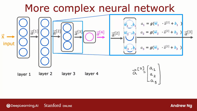
Each NN layer takes an input and returns an output. This output is called the activation value and is calculated using this formula:
Where g is the sigmoid function, also called activation function, and the parameters are taken from the logistic regression formula:
This returns an activation value that forms a vector if we have more than one neuron:
This vector is taken as input for the next layer
The activation value recieves a subscript that denotes the layer in which was obained, so the second layer will have this formula:
If we only have one neuron the return will be a scalar value
a = 0.82
The last step which is optional is a classification process for which we need to set a threshold:
is a >= 0.5
yes: y = 1
No: y = 0
The general formula for the activation value is:
The below graph shows the general architecture of a complex NN that use the above formula on each of the layers and neurons
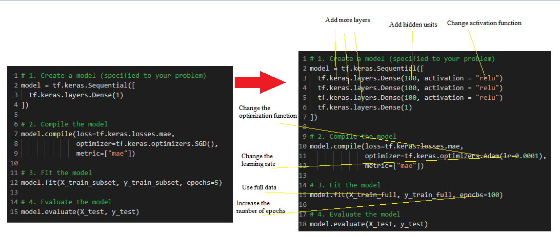
The common ways to improve a model are:
- Adding layers
- Increase the number of hidden units
- Change the activation functions
- Change the optimization function
- Change the learning rate (This is perhaps the most important parameter)
- Fitting on more data
- Fitting for longer
We must go through each of these individually and adjust as we see the results.
Sometimes the model with more layers, a small learning rate, and a high number of epochs is not the best one, so that's why we need to keep evaluating each metric one by one and see what works.
Natural Language Processing
We need to change each word to a numerical value. The dataset used is a review of movies from the TensorFlow library. All reviews must have the same length, so the data needs to be standardized. The way it works is by:
- if the review is greater than 250 words, then trim off the extra words
- if the review is less than 250 words, add the necessary amount of 0's to equal 250.
Which can be achive by using
from keras.preprocessing import sequence
train_data = sequence.pad_sequences(train_data, 250)
This is the overall look of the model for NLP
The Embedding layer find a more meaningfull representation of our current data into vectors of 32 dimensions We Long Short Term Memomry for our neurons (so they can learn from the previous output) The activation function is the sigmoid function which allow to have a value between 0 and 1
model = tf.keras.Sequential([
    tf.keras.layers.Embedding(VOCAB_SIZE, 32),
    tf.keras.layers.LSTM(32),
    tf.keras.layers.Dense(1, activation="sigmoid")
])
We train the data by setting up the parameters of the loss function, the optimizer, and the metrics
model.compile(loss="binary_crossentropy",optimizer="rmsprop",metrics=['acc'])
We pass the training data, the epochs and choose the amount of data use for the validation data
history = model.fit(train_data, train_labels, epochs=10, validation_split=0.2)
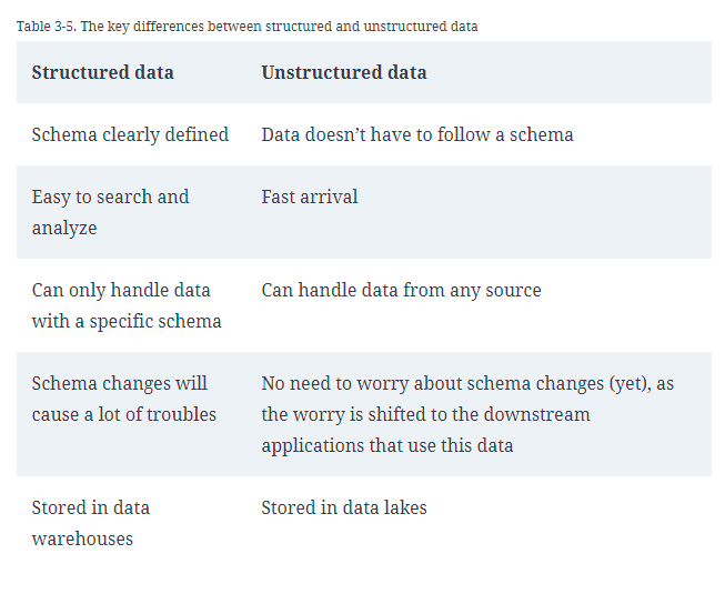
The above table shows the difference between Strcuture data and unstructure data. This is a critical aspect of ML systems since is going to decide how are we going to store our data and provide to the different departments.
Unstructured data allow flexibility. If things on the data change, we can easily customize with unstructured data since all our data doesn't need to follow the same schema. On the other hand, structure data follows the same schema, so if one thing changes, all the data needs to be customized to incorporate the change. Usually, structured data is used to store data that has been processed and sent to the teams for analysis, while non-structured data is raw data that needs some type of transformation.
Types of workloads:
- Transactional Processing
- Analytical Processing
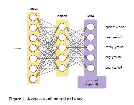
Often, we might need to classify things with one or more labels. This can be achieved with the One vs. all approach to leverage binary classification, in which we create a binary classifier for each possible outcome.
This approach is reasonable with a few classes but becomes increasingly inefficient as the number of classes rises.
The second approach is Softmax in which we extend the idea of the logistic regression into a multiclass world.
Softmax options
-Full softmax: calculates the probability for every possible class -Candidate sampling: means that softmax calculates a probability for all possible labels but only for a random sample of negative labels. This approach can improve efficiency with large number of classes.
Softmax assumes that each example belong to exactly just one class, however if the problem has more than one class you may not use softmax and you most rely on multiple logistic regressions.
To access to the pictures in a dataset after each picture is code by a number you can use:
matplotlib.pyplot.imshow which allow to interpret numeric array as an image
# import modules
import numpy as np
import pandas as pd
import tensorflow as tf
from tensorflow.keras import layers
import matplotlib.pyplot as plt

# get the mnist dataset
(x_train, y_train),(x_test, y_test) = tf.keras.datasets.mnist.load_data()

# Show image
plt.imshow(X_train[2917])
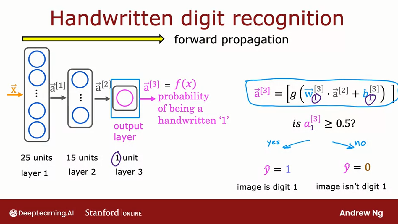
Forward propagation is a sequence of steps in Neural Networks to return an output.
These are the step for build a NN:
- Select the number of hidden layers
- Select the neurons in each hidden layer
Behind scenes the calculation will be the activation value in each layer that will serve as input for the next layer, this type of sequential steps is called forward propagation.
Evaluating a TensorFlow model
For evaluating a TF model we need to visualize
- The data - what data are we working with? What does it look like?
- The model itself - what does our model look like?
- The training of a model - how does a model perform while it learns?
- The predictions of the model - how do the predictions of a model line up against the ground truth
Transactional databases are designed to have low latency and high availability requirements. Transactional databases has 4 characteristics:
- Atomicity: All steps in a transaction are completed as a group
- Consistency: All transactions must follow predefined rules
- Isolation: To guarantee that two transactions happen at the same time
- Durability: To guarantee that once a transaction has been committed, it will remain committed even in the case of a system failure.
An interesting paradigm in the last decade has been to decouple storage from processing (also known as compute), as adopted by many data vendors including Google’s BigQuery, Snowflake, IBM, and Teradata. In this paradigm, the data can be stored in the same place, with a processing layer on top that can be optimized for different types of queries.
NLP allows evaluating the sentiment of words in a sentence by converting them into integers. The output is a numerical value between 0 and 1 that denotes the probability of a positive sentence. We can add a threshold to our decisions to classify them into positive or negative.
Embeddings Allow you ow to transform your data into numerical values and represent them as numerical values, from which you can calculate how similar they are based on location in a multidimensional space. Embeddings make it easier to do ML on large inputs.
One thing to remember is that the dimensions representing your data are hyperparameters that can be optimized. As a rule of thumb, you want to apply the fourth root of the possible values in our outcome.
-Higher dimesional embeddings can represent accurately the representation between input values
-More dimensions increase the chance of overfitting and leads to slower training
To obtain the activation values in Python we can do the following:
The following code returns the activation value for a layer with 3 neurons and use the sigmoid function as activation function. The second layer
x = np.array([[200.0, 17.0]])
layer_1 = Dense(units=3, activation="sigmoid")
a1 = layer_1(x)

layer_2 = Dense(units=1, activation="sigmoid")
a2 = layer_2(a1)
Data in TensorFlow
Let's start on how numpy represents the data
| temperature | duration | Good coffe? (1/0) |
|---|---|---|
| 200.0 | 17.0 | 1 |
We have temperature and duration as independent feature, those can be represented in a NumPy array in different ways:
x = np.array([[200.0, 17.0]])
To explain why we have two square brackets we need to understand how numpy stores data
This is a bidimensional 2 x 3 matrix. It has 2 rows and 3 columns
NumPy representation of the same matrix is:
x = np.array([[1,2,3],
             [4,5,6]])
This is a bidemensional 4 x 2 matrix
NumPy representation of this matrix is:
x = np.array([[0.1, 0.2],
              [-3.0, -4.0,],
              [-0.5, -0.6],
              [7.0, 8.0]])
Going back to the problem, there are different ways to represent the same information:
x = np.array([[200.0, 17.0]]) # creates a 1 by 2 matrix: 1 row and 2 columns

x = np.array([[200],
               [17]]) # creates a 2 by 1 matrix: 2 rows 1 column

x = np.array([200,700]) # creates a 1-d vector
TensorFlow has the convention to store the data in matrix and not in vectors which is something to be aware while working with these two libraries.
The three sets...
Training set - the model learns from this data (70-80%)
Validation set - The model gets tuned on this data (10-15%)
Test set - The model gets evaluated on this data (10-15%)
Split your data
X_train = X[:int(len(X)*0.8)]
y_train = y[:int(len(X)*0.8)]

X_test = X[int(len(X)*0.8):]
y_test = y[int(len(X)*0.8):]
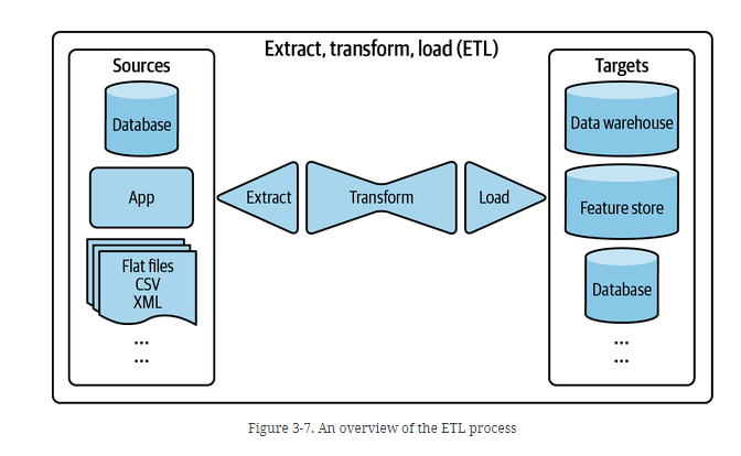
E: Extract the data from all your data sources - Validate your data and reject the one that doesn't meet the requirements
T: Transform might imply join data, clean it. Standardize value ranges, apply operation and derive new features.
L: Load is deciding how often to load your transformed data into the target destination.
Text generator allows to predict the next character using length of a sequence as input.
For this we need to create a dictionary with every unique character in our text that encodes every character with a number, so each word will have a unique sequence of numbers.
Since we want to predict the next character based on a length sequence we need to split our data. e.g. Input: Hell | output: ello
We use a batch approach which mean we are not going to do this for every word instead we will be using this for a batch of words.
Machine Learning systems has a wide of range of components that are not part of the training system of your data
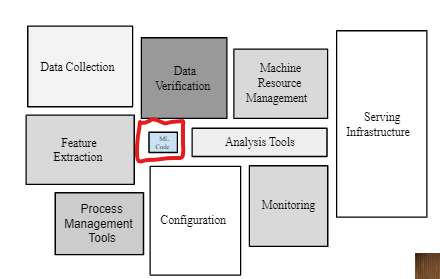
The above picture shows the requirements for ML model in production, some systems design can help in many of these components.
Building a Neural Network architecture in TensorFlow
model = Sequential([
    Dense(units=25, activation="sigmoid"),
    Dense(units=15, activation="sigmoid"),
    Dense(units=1, activation= "sigmoid")])

model.compile(...)

x = np.array([[0..., 245, ..., 17], # x is a multidimensional matrix
      [0..., 200, ..., 184])

y = np.array([1,0]) # y is an 1d array
model.fit(x, y)

model.predict(x_new)
Let's define a model just using the shape of our tensors and not the actual data
model = tf.keras.Sequential([
    tf.keras.layers.Dense(1, input_shape=[1])
])

model.compile(loss=tf.keras.losses.mae,
    optimizer=tf.keras.optimizers.SGD(),
    metrics=["mae"])
When we evaluate this model it has three notable things:
- Total params: total number of parameters in the model
- Trainable parameters - these are the parameters (patterns) the model updates as it trains
- Non-trainable parameters: these parameters aren't updated during training (this is typical when you bring in already learn patterns or parameters from other models during transfer learning
There are three main process for data flow:
Data Passing Through Databases
Pros: Easiest way to pass data betwee process Cons: Both processes must be able to access the same database (not always feasible if process are run by different companies) - It might be a slow process
Data Passing Through Services
Passing data directly to a network and different companies with different purpose can run the data at the same time
The most popular styles of requests used for passing data through networks are REST (representational state transfer) and RPC (remote procedure call). “REST seems to be the predominant style for public APIs. The main focus of RPC frameworks is on requests between services owned by the same organization, typically within the same data center.”
Data Passing Through Real-Time Transport
Real Time transport allow to request and get data from multiple services using a Broker to coordinate data among services.
The most common types of real time transport are:
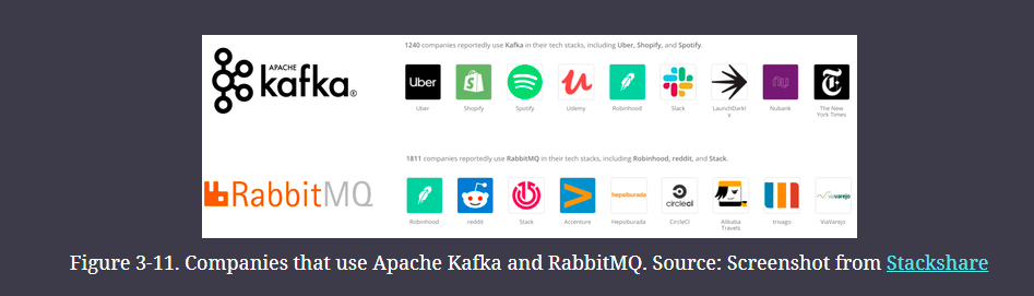
-pubsub in which any service can publish and subscribe to a topic, pubsub often have a retention policy, the data is retained for a certain period before deleted or move to a permanent storage (e.g. Apache Kafka and Amazon Kinesis)
-Message queue model
In a message queue model, an event often has intended consumers (an event with intended consumers is called a message), and the message queue is responsible for getting the message to the right consumers (e.g. Apache RocketMQ and RabbitMQ)
Historical data is processed in batch jobs (once a day) -> Batch processing (e.g. MapReduce and Spark)
Streaming data - real time transport (Apache Kafka and Amazon Kinesis)
Streaming can use technologies like Apache Flink. In stream processing you can just compute the new data and joining the new data computation with the older data computation.
Batch processing can be used for static features (don't change often) while stream processing for dynamic features (change often)
Static: offine vs. Dynamic training
Static: Trained just once
- Easy to build and test -- use batch train & test, iterate until good
- Requires monitoring inputs (if the distribution of input changes and our model is not adapted is likely to underperform)
- Easy to let this grow stale (need to retrain if new conditions are place)
Dynamic: Data comes in and we incorporate that data into the model through small updates
- Continue to feed in training data over time, regularly sync out updated version
- Use progressive validation rather than batch training & test
- Needs monitoring, model rollback & data quarantine capabilities
- Will adapt to changes, staleness issues avoided
In python:
w = np.array([[1, -3, 5]
              [2, 4, -6]])

b = np.array([-1, 1, 2])

a_in = np.array([-2, 4]) # could be a_0 which is equal to x

def dense(a_in, W, b, g):

    units = W.shape[1] # columns of the w matrix = 3
    a_out = np.zeros(units) # [0,0,0]

    for j in range(units): # 0,1,2
        w = W[:,j]
        z = np.dot(w, a_in) + b[j]
        a_out[j] = g(z)

    return a_out

def sequential(x):

    a1 = dense(x, W1, b1)
    a2 = dense(a1, W2, b2)
    a3 = dense(a2, W3, b3)
    a4 = dense(a3, W4, b4)
    f_x = a4
    return f_x
Vectors can be represented as transpose vector, in which from column vector we can have a row vector and the results will be the same
Is equal to:
We dfine the W matrix
Matrix transpose takes the columns and converted into rows
row1 col1
row2 col1
row1 col2
row2 col2
Vectorize Implementation
AT = np.array([[200, 17]])

W = np.array([[1, -3, 5],
              [-2, 4, -6])

b = np.array([[-1, 1, 2]])

def dense(AT, W, b, g):

    z = np.matmul(AT, W) + b
    a_out = g(z)

    return a_out
- Specify how to compute output given input X and parameters w and b
- Specify the loss and cost
- Train on data to minimize the cost function
Logistic regression steps
z = np.dot(w, x) + b
f_x = 1/(1+np.exp(-z))
loss = -y * np.log(f_x) -(1-y) * np.log(1-f_x)
w = w - alpha * dj_dw
b = b - alpha * dj_db
Neural Network steps
import tensorflow as tf
from tensorflow.keras import Sequential
from tensorflow.keras.layers import Dense
model = sequential([
	    Dense(units = 25, activation = "sigmoid")
	    Dense(units=15, activation = "sigmoid")
	    Dense(units=1, activation = "sigmoid")
			    ])
# binary prediction
from tensorflow.keras.losses import BinaryCrossentropy
model.compile(loss = BinaryCrossentropy())

# regression prediction
from tensorflow.keras.losses import MeanSquaredError
model.compile(loss = MeanSquaredError())
# Minimize the cost function using back propagation
model.fit(X, y, epochs=100)
TensorFlow allows visualizing the model and customize the names for a better explanation on how we build the model.
Let's use an example without data by using just the input shape of the model:
import tensorflow as tf
# build the model
model = tf.keras.Sequential([
tf.keras.layers.Dense(10, input_shape=[1], name="input_layer"),
tf.keras.layers.Dense(1, name="output_layer")
], name="model_1")

# compile the model
model.compile(loss=tf.keras.losses.mae,
optimizer=tf.keras.optimizers.SGD(),
metrics=["mae"])

model.summary()
This creates a model summary with layers, the output shape of each layer, and the parameters. The total parameters divided by the trainable parameters and non-trainable parameters.
Plot the model
from tensorflow.keras.utils import plot_model
plot_model(model=model, show_shapes=True)Feedback loop: It is defined as the time from when a prediction is served until when feedback is provided.
Short feedback loops are task where labels are generally available within minutes (e.g. recommendation system for streaming services, stock market...)
Long feedback loop are task where labels are available for weeks or even months (e.g. fraud detection systems...)
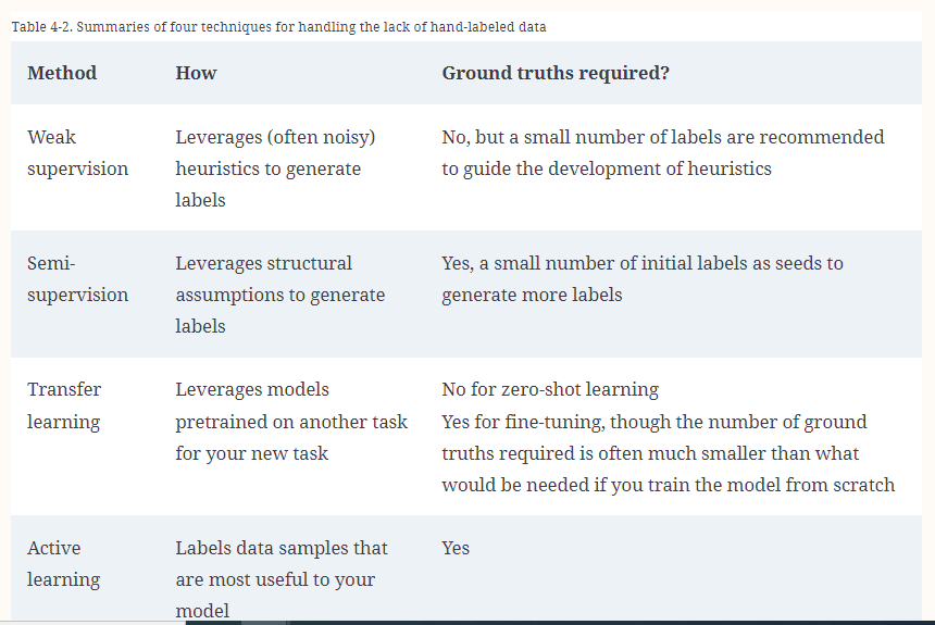
There are four types of method for lack of labels, summarize in the below table.
NLP has several steps to follow for building a model:
- Start by decoding your text into numbers
- Separated between training and testing example
- Choose the first parameters of your model
- Build the model (use embedding layer, LSTM layer and the output layer)
- Create the loss function
- Compile the model
- Generate text
Data is the most important asset of the models, we need to evaluate features using a check list:
- Reliability: What happens when the signal is not available?
- Versioning: Does the system that computes this signal ever change?
- Necessity: Does the usefulness of the signal justify the cost of including it?
- Correlations: are the features causal or just correlated? will this relationship change over time?
- Feedback Loops: which of my input signals may be impacted by my model's outputs?
Activation Functions
There are three activations functions that we can use in many ways to came up with powerful models:
Let's breakdown by layers:
Output layer
Linear activation functions: Better for values that can take positive and negative values Sigmoid functions: Better suit for binary classification problems ReLU: Better for positive numbers such as house price
Hidden layer ReLU is the most common activation function for the hidden layers since it provide a faster learning. The explanation behind this statement is that ReLU is flat on just one side of the graph while sigmoid is flat in both places which make gradient descent converge in a slower pace.

The code implementation of the above theory is:
from tf.keras.layers import Dense
model = Sequential([
	Dense(units=25, activation='relu'),
	Dense(units=15, activation='relu'),
	# for binary output
	Dense(units=1, activation='sigmoid')
])def plot_predictions(train_data=X_train,
train_labels=y_train,
test_data = X_test,
test_labels=y_test,
predictions=y_pred):
"""
Plots training data, test data
"""
plt.figure(figsize=(10,7))
# plot training data in blue
plt.scatter(train_data, train_labels, c="b", label="Training data")
# plot testing data in green
plt.scatter(test_data, test_labels, c= "g", label="Testing data")
# plot model predictions in red
plt.scatter(test_data, predictions, c= "r", label="Predictions")
# show legend
plt.legend();Terminology: Environment: Learning task that our agent explore Agent: Entity that explore the environment State: Status of the agent (e.g. location in the environment) Action: Interaction between the agent and the environment Reward: Every action that our agent takes will result in a reward (positive or negative)
Q-Learning Possible actions that can be performed by the agent in a given step with the expected return
Type of Bias
- Reporting bias
- Automation bias
- Selection bias
- Group Attribution bias
- Implicit bias
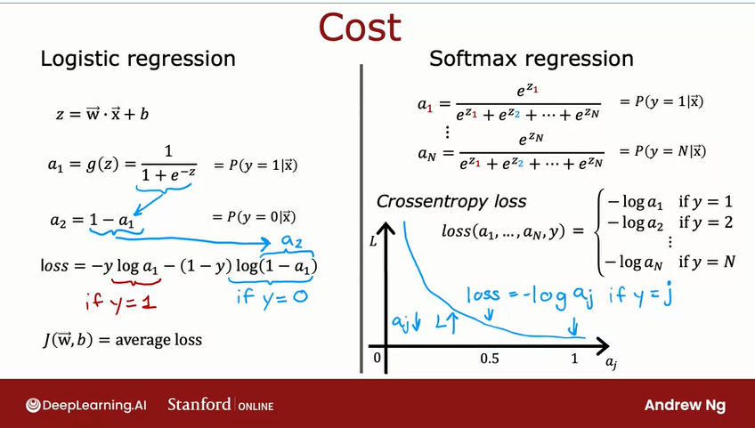
Softmax:
Logistic regression returns the probability of y = 1, therefore it also returns the probability of y = 0
Let's review an example
Softmax regression for 4 possible outcomes
-
$$ z_1 = w_1 * x + b_1 $$
-
$$ z_2 = w_2 * x + b_2 $$
-
$$ z_3 = w_3 * x + b_3 $$
-
$$ z_4 = w_4 * x + b_4 $$
The formula to compute the probability of y in each outcome is computed by using:
-
$$ a_1 = {e^{z1}\over e^{z_1} + e^{z_2} + e^{z_3} + e^{z_4}} = P(y = 1|x) $$
-
$$ a_2 = {e^{z2}\over e^{z_1} + e^{z_2} + e^{z_3} + e^{z_4}}= P(y = 2|x)$$
-
$$ a_3 = {e^{z3}\over e^{z_1} + e^{z_2} + e^{z_3} + e^{z_4}}= P(y = 3|x) $$
-
$$ a_4 = {e^{z4}\over e^{z_1} + e^{z_2} + e^{z_3} + e^{z_4}}= P(y = 4|x) $$
General formula based on these assumptions:
Cost function
Neural Network with softmax output
The hidden layers are calculated following the same rules of the previous examples.
The output layer is calculated using softmax to get the probabilities of each one of the classes.
The Python code for a multi-classification problem is:
- Specify the model:
# 1- specify the model
import tensorflow as tf
from tensorflow.keras import Sequential
from tensorflow.keras.layers import Dense
model = Sequential([
	Dense(units=25, activation='relu'),
	Dense(units=15, activation='relu'),
	Dense(units=10, activation='softmax')
])- Specify the loss and cost
from tensorflow.keras.losses import SparseCategoricalCrossentropy
model.compile(loss=SparseCategoricalCrossentropy())- Train on data to minimize J(w,b)
model.fit(X, Y, epochs=100)This is not the most efficient way of implementing the code since some numerical errors might occur, the most efficient way is:
import tensorflow as tf
from tensorflow.keras import Sequential
from tensorflow.keras.layers import Dense
model = Sequential([
	Dense(units=25, activation='relu'),
	Dense(units=15, activation='relu'),
	Dense(units=10, activation='linear')
	])
from tensorflow.keras.losses import SparseCategoricalCrossentropy
model.compile(loss=SparseCategoricalCrossentropy(from_logits=True))
model.fit(X, Y, epochs=100)
logits=model(X)
f_x =tf.nn.softmax(logits)Advance Optimization
Adam algorithm
Allow to optimize the convergent rate of gradient descent by increasing or decreasing alpha automatically.
Adam: Adaptive Movement estimation
Python implementation of ADAM
# Model
model = Sequential([
		tf.keras.layers.Dense(units=25,activation="sigmoid"),
		tf.keras.layers.Dense(units=10,activation='sigmoid'),
		tf.keras.layers.Dense(units=10,activation='linear')
# compile
model.compile(optimizer=tf.keras.optimizers.Adam(learning_rate=1e-3),
	loss=tf.keras.losses.SparseCategoricalCrossentropy(from_logits=True))
#fit
model.fit(X,Y, epochs=100)Evaluation metrics
There are different evaluation metrics depending on the problem you're working on.
- MAE - mean absolute error: on average how wrong is each of my model's predictions
- MSE - mean square error, "Square the average errors"
| Metric name | Metric formula | TensorFlow code | When to use |
|---|---|---|---|
| Mean absolute error (MAE) |
tf.keras.losses.MAE() or tf.metrics.mean_absolute_error()
|
As a great starter metric for any regression problem | |
| Mean square error (MSE) |
tf.keras.losses.MSE() or tf.metrics.mean_square_error()
|
When larger errors are more significant than smaller errors. | |
| Huber | tf.keras.losses.Huber() |
Combination of MSE and MAE. Less sensitive to outliers than MSE. |