LGD 17/12/2021
- Quick start
- Detailed examples
- Dataset 1: Rainfall and river flow
- Dataset 2: Cell and nucleus
- Downstream analysis: ERK and AKT data mining
This is a package for detecting and visualising correlations between objects in biological series data.
Citation
lifeTimes is available for everyone. If you find it useful for your research please cite the work that motivated its development: Environmentally dependent and independent control of cell shape determination by Rho GTPase regulators in melanoma. doi: https://doi.org/10.1101/2021.10.11.463377
Install lifeTimes
#install devtools if needed
if(!require("devtools")) install.packages("devtools")

#load devtools
library(devtools)

#install dependency from github
if(!require("ComplexHeatmap")) install_github("jokergoo/ComplexHeatmap")

#install lifeTimes from github
install_github("somaSystems/lifeTimes")
Run lifeTimes on default data
#copy and paste to run on test data
library(lifeTimes)
# rm(lifeTimes)

lts <- lts_in() #calculate cross correlation
Visualise results from lifeTimes on default data
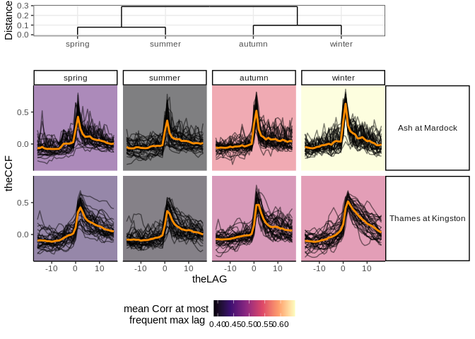
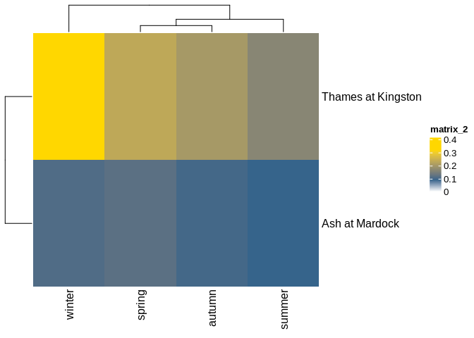
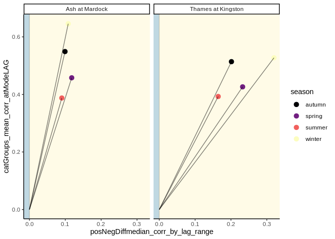
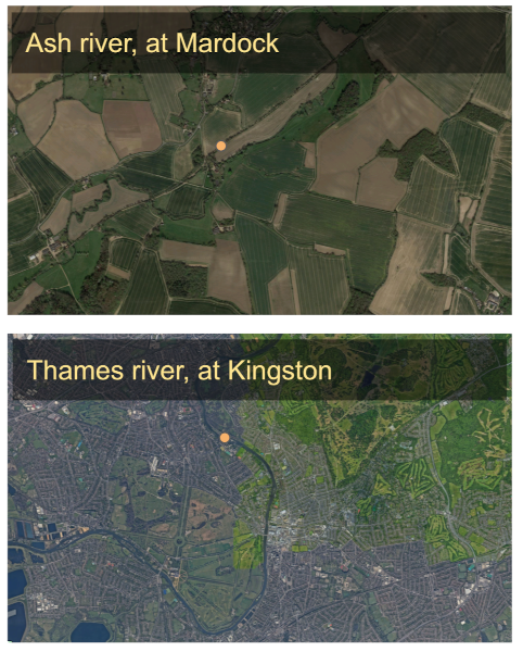
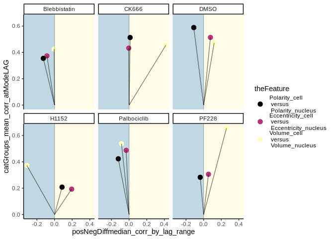
lts_plot_ccfs(lts) #plot clustered correlationslts_plot_ClustSum(lts) #plot direction of correlationslts_plot_coupled(lts) # plot strength and direction of correlationFig 1 Ariel images of the Ash, and Thames rivers.
Fig 1: Ariel images of the Ash, and Thames riversQuick summary on inputs
i. Evenly spaced series data (eg. can be time or space series)
ii. Label of the measurements taken. (eg. can be shape or signal
intensity)
iii. Labels for the objects to be compared (eg. cytoplasm and nuclear
compartments)
iv. Higher level groupings for comparing objects (eg. compare objects
per cell/organism/treatment/community)
Quick notes on outputs
i. Plots of calculated correlations clustered by strength at lag zero
ii. Plots of calculated asymmetries between past and future lags,
clustered by strength of asymmetry
iii. Plots representing both the strength of correlation at lag zero,
and the direction of correlation
iv. Calculated summary statistics of CCFs that can be used in downstream
analysis (e.g to improve the performance of classification tasks)
description of default data lifeTimes makes it easy to detect
“coupling” between different components of biological systems from the
scale of cells, to organisms, to ecosystems. Along these lines,
lifeTimes comes with examples of:
i.landscape scale datasets, ii.subcellular scale datasets.
Landscape scale data lifeTimes can be used to find coupling between processes at the landscape or ecosystem scale. For this example, I have used data from the United Kingdom, National River Flow Archive (https://nrfa.ceh.ac.uk/web-download-service). We will look at two types of data, i) Gauged Daily Flows (GDF) which measure how much water is in a river, and ii) Catchment Daily Rainfall (CDR) which measure the amount of rain on the landscape around the river. River flows are in cubic meters per second, and rainfall is in mm across the catchment in the given reference period (https://nrfa.ceh.ac.uk/data-formats-types).
For this example I have downloaded data from the Thames river, at Kingston (), and the Ash river, at Mardock . I have also subset the data between the years 1983 and 2017. This is a period where both stations were operating, and recording measurements.
After some data wrangling, these two datsets produce a csv which I read into a dataframe. The first five observations look like this:
rain_flow <- read.csv(file ="data-raw/rain_flow_Thames_Ash.csv")
head(rain_flow)
## date dateAsInteger catchmentRegion flow_m3s rainfall_cm year month day
## 1 1983-06-01 4899 Ash at Mardock 4.720 3 1983 6 1
## 2 1983-06-02 4900 Ash at Mardock 0.756 12 1983 6 2
## 3 1983-06-03 4901 Ash at Mardock 0.543 8 1983 6 3
## 4 1983-06-04 4902 Ash at Mardock 0.450 0 1983 6 4
## 5 1983-06-05 4903 Ash at Mardock 0.392 0 1983 6 5
## 6 1983-06-06 4904 Ash at Mardock 0.363 0 1983 6 6
## yearNumber dayNumber Reset_SeasonYearDay dayOfYear season dayOfseason
## 1 1 365 0 0 summer 0
## 2 1 366 1 1 summer 1
## 3 1 367 2 2 summer 2
## 4 1 368 3 3 summer 3
## 5 1 369 4 4 summer 4
## 6 1 370 5 5 summer 5
## catchRep uniqueID key_num
## 1 year_1_Ash at Mardock 1Ash at Mardocksummer key_83
## 2 year_1_Ash at Mardock 1Ash at Mardocksummer key_83
## 3 year_1_Ash at Mardock 1Ash at Mardocksummer key_83
## 4 year_1_Ash at Mardock 1Ash at Mardocksummer key_83
## 5 year_1_Ash at Mardock 1Ash at Mardocksummer key_83
## 6 year_1_Ash at Mardock 1Ash at Mardocksummer key_83
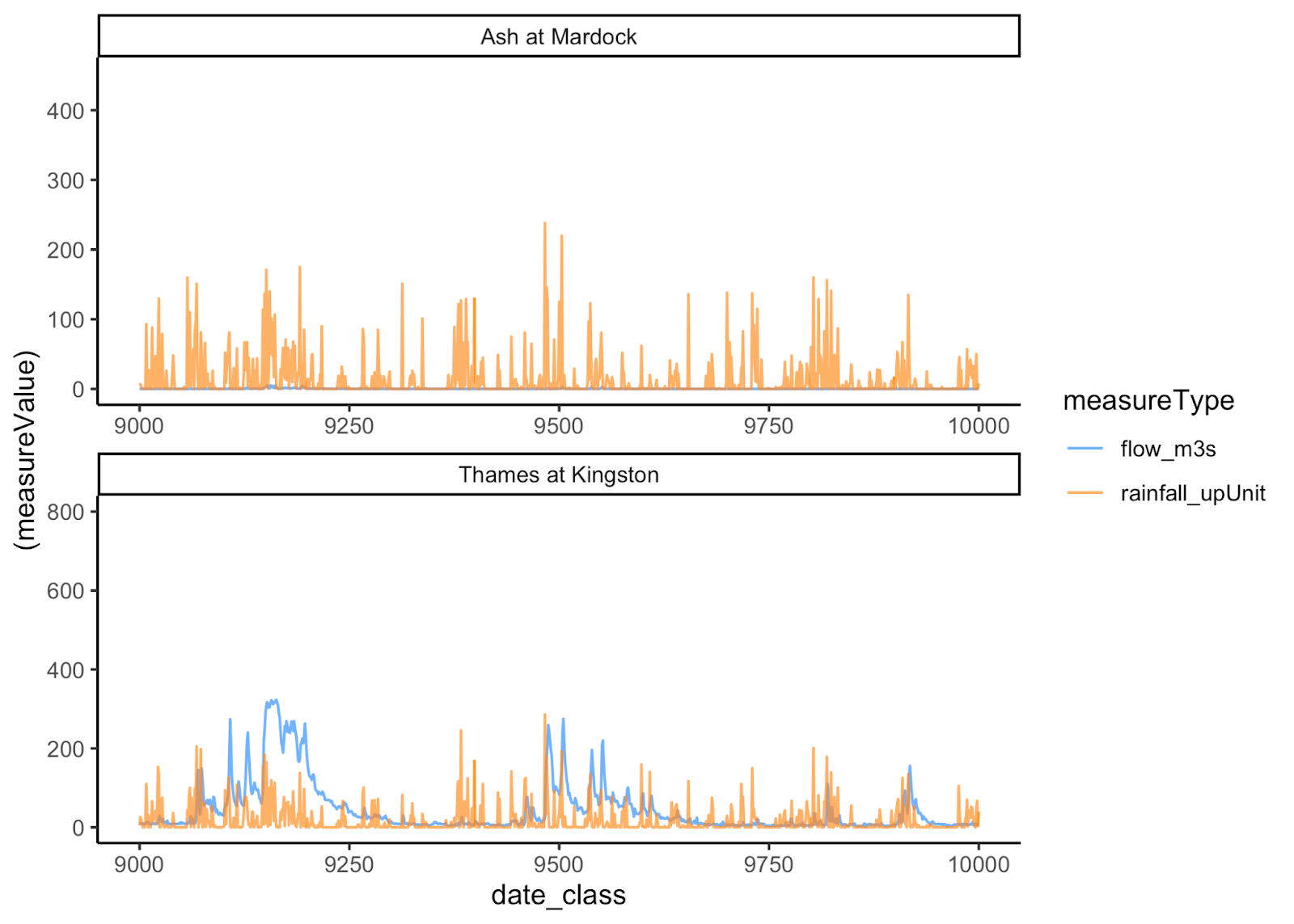
Plotting the river flow and rainfall measures over a 1000 day interval
looks like this:
The main funtion for user input in lifeTimes is lts_in(). To test that
lifeTimes is working you can run this function without any arguments.
This will run the program on a default set of data.However, it is more
interesting to run lifeTimes on your own data. Below, I have included a
worked example of how to use run lifeTimes on a dataset. For this
example, I am still usingthe rain_flow dataset, except that the steps
to run this data in lts_in() are now clearly shown.
Example 1
library(lifeTimes) #load lifeTimes namespace

#use the lts_pairsMaker hrlper function
#to prepare variables to be compared in a list of lists format
lts_pairedVars <- lts_pairsMaker(c("rainfall_cm","flow_m3s"))
lts_pairedVars
## $rainfall_cm
## $rainfall_cm[[1]]
## [1] "rainfall_cm"
##
## $rainfall_cm[[2]]
## [1] "flow_m3s"
#arguments for lts_in() with default inputs (the "river catchments "rain_flow" dataset) shown
lts_in(.in_tsData = rain_flow  , #1. the dataset
         .in_time = c("dayOfseason"), #2. the time column
       .in_compare_categorical =  c("season", "catchmentRegion"), #3. A vector, with the names of categorical columns
       .in_plot_measured_variables = FALSE , #4. Whether to CCFs for multiple pairs of variables
       .in_pairedComparisons =  list(pair_1 = list(y = "rainfall_cm",
        x = "flow_m3s")), #5. A list of lisys, holding the pairs of variables to be compared
       .in_uniqueID_colname = "key_num", #6. The column with unique ID name for your observations
       .in_metaData = NULL) #7. Column names of any attributes you would like to append to data
I will now give a walkthrough that explains the arguments above, and how to run lifeTimes, on your own data! To make any data suitable for lifeTimes, we need the raw data, and four types labels which identify the “time”,“unique ID”, “categorical variable” and “measured variable” columns. There is also an option to identify metadata:
The Arguments
1:.in_tsData = A series dataframe: Time series measurements. These
should have:
i. at least two variables,
ii. evenly spaced intervals,
iii. Complete sets of observations (e.g NAs, can be imputed).
iv. Time series of equal length.
v. At least two categorical variables (e.g Treatment vs Control)
TODO: lifeTimes will be compatible with orical variable, and missing observations. A helper function to impute NAs will also be included.
2: .in_time = A unit of time: So we need to find the column in the
dataset that indicates this. In this data we have years, months and
days, but the unit of time I am interested in is at the resolution of
days. The column in the datset with days is called "dayOfseason". On
the first day of each season (summer, autumn, winter, spring) this value
starts at one and increments up until the end of the season.
3: .in_compare_categorical = Categorical Variables: This is where
you tell lifeTimes which colums hold the labels for categorical
variables. For example these might be experimental treatments or
conditions. Currently you can have 1 or 2 categorical variables. For the
rainflow dataset there are 2 columns with categorical variables, and
they are “season” (e.g a label that is ‘summer’, ‘autumn’, ‘winter’ or
‘spring’) and “catchmentRegion” e.g “Ash at Mardock” or “Thames at
Kingston”. LifeTimes will cluster your categorical data based on
correlations between measured variables.
4: .in_plot_measured_variables = Whether to plot multiple
variables? This parameter takes a logical argument and can be either
“TRUE” or “FALSE”. The choice depends on whether you are analysing two
categorical variables, in which case set it to “FALSE”. If you are
studying one categorical variable but would like to calculate and plot
the cross correlations of multiple mesured variables, set this to
“TRUE”. A detailed explanation is below.
Currently in lifeTimes, categorical and measured variables can be used in two ways:
- You can analyse 2 categorical variables and one pair of measured variables. This is shown with the “rain_flow” dataset. The two categorical variables are “catchment” and “season”, and the pair of measured variables are “rainfall_cm” and “flow_m3s”.
- alternatively, if you are using one categorical variable, but more
than one pair of measured variablesyou can set this to
.in_plot_measured_variables = TRUE
5: .in_pairedComparisons = Pairs of variables to compare to one
another at different lags: Under the hood, these are passed to the
lifeTimes internal functions in the format of a list of lists. There is
one master list, holding lists of paired variables to compare. In
practice, there is a helper fuction lts_pairsMaker(), that takes a
vector with a list of column names, and returns all possible non
redundant pairs of variables in this list. So you can give a list of
variables you would like to compare to the lts_pairsMaker function,
and assign the output to an object. Then just pass this object as an
argument to the .in_pairedComparisons = parameter (See example 1
above). In addition to iterating all possible combinations of pairings
between variables, lts_pairsMaker can be passed a table of
pre-specified pairings, and return these in list of list format (this is
demonstrated in the examples below).
6:.in_uniqueID_colname = A unique identified for each thing we are
measuring: We need to give lifeTimes the column namr which holds the
unique identifier for each observation. If there isn,t one, we can
create a column in the data frame with unique identifier for each
observation.
In this dataset the column is called “key\_num”. In general, an unit of observation is some unit of interest, measured over time. In this dataset, it’s a river measuring station, in a given season, in a given year. For example, “Ash river in summer in 1995”, or “Thames river in winter of 2001”. So in this dataset I have grouped the data by, River,Season and Year, and given a unique ID to each observation and labelled the column `"key_num"`.
TODO: Future updates to lifetimes will include a helper function that inputs a set of columns defining a unique observation, and outputs creates a new column of uniqueIDs.
7: .in_metaData = Column names of metadata: This parameter takes
column names of any attributes you would like to append to data
Subcellular scale data We have seen that lifeTimes can be used to detect the coupling between lanscape scale processes such as rainfall and riverflow, and to highlight how this coupling varies between seasons and geographical regions. In this next example, I am using lifeTimes to look at coupling between the overall geometry of a living cell, and the nucleus compartment within that cell. For this example I have used data from melanoma cells imaged in a 3D collagen matrix, treated with different drugs that affect cell function. The data here are just 30 cells (5 cells for each drug treatment), sampled for demonstration purposes, from a larger dataset.
First I read in the ‘sampleCells.csv’ data, that is included in the lifeTimes package.
###start example
lts_cells <- read.csv(file = "data-raw/sampleCells.csv")
Next, I look at the column names to see the categorical variables, and measured variables in the dataset
#look at colum names
colnames(lts_cells)
## [1] "Volume_cell" "EquivDiameter"
## [3] "SurfaceArea_cell" "MeanIntensity"
## [5] "MinIntensity" "MaxIntensity"
## [7] "MajorAxis_cell" "MinorAxis_cell"
## [9] "secondMajor_cell" "Eccentricity_cell"
## [11] "secondEccentricity_cell" "Sphericity_cell"
## [13] "Vol2surf_cell" "runNumber"
## [15] "timeTrack" "yDim"
## [17] "xDim" "zDim"
## [19] "xCoord_cell" "yCoord_cell"
## [21] "zCoord_cell" "Orbit"
## [23] "AngleBetween" "serialNumber"
## [25] "nProtrusions_cell" "CoverslipPresent"
## [27] "CoverslipDistance" "OnCoverslip"
## [29] "fieldNumber" "Treatment"
## [31] "Row" "Column"
## [33] "Polarity_cell" "Spreading_cell"
## [35] "Protrusivity_cell" "cellNumber"
## [37] "NucleusVolumeFraction" "Volume_nucleus"
## [39] "SurfaceArea_nucleus" "MajorAxis_nucleus"
## [41] "MinorAxis_nucleus" "secondMajor_nucleus"
## [43] "Eccentricity_nucleus" "secondEccentricity_nucleus"
## [45] "Sphericity_nucleus" "Vol2surf_nucleus"
## [47] "xCoord_nucleus" "yCoord_nucleus"
## [49] "zCoord_nucleus" "nProtrusions_nucleus"
## [51] "Polarity_nucleus" "Spreading_nucleus"
## [53] "Protrusivity_nucleus" "Plate"
## [55] "cluster"
Here, I can see that "runNumber", will be the column with the time
information, and "cellNumber" will be the unique ID for each
observation. "Treatment" is a categorical variable.
For this dataset, I am only interested in one categorical variable, called “Treatment”. This variable describes the drug that each cell has been exposed to. This is in contrast to the “rain\_flow” dataset (example 1 above) where there were two categorical variables of inerest (“season” and “catchmentRegion”).
Also, I can see that there are many measured variables for both the cell and nucleus that I could compare (eg. “Polarity\_cell”, “Eccentricity\_nucleus”, “Volume\_cell” etc.) . This is in contrast to the “rain\_flow” dataset where there were only two measured variables.
User defined paired comparisons For this dataset, instead of using
lts_pairsMaker to permute all the possible comparisons between
measured variables, I will specifically define the variables to compare.
In the cell dataset, we can use some domain specific knowledge to
recognise that comparing the coupling of geometry between the cell and
nucleus under different drug treatments is meaningful and interesting.
To make this comparisons, I have just listed some of the features I
would like to directly compare, and then joined this into a matrix that
I named my_pairs by using rbind():
#choose three pairs of column names
pair1 <- c("Polarity_cell","Polarity_nucleus")
pair2 <- c("Eccentricity_cell", "Eccentricity_nucleus")
pair3 <- c("Volume_cell", "Volume_nucleus")

# use rbind to make these pairs into a matrix
my_pairs <- rbind(pair1,pair2,pair3)
I passed my_pairs to lts_pairsMaker with defined = TRUE, to create
a list of specific paired comparisons that I would like to make. This
contrasts with the less default use of lts_pairsMaker, where a list of
column names is entered, and all possible non-redundant combinations of
these are returned.
#make these into list of pairs using helper function with "defined = TRUE"
lts_pairs <- lts_pairsMaker(my_pairs, defined = TRUE)
The data, relevant column names and list of pairs can all be entered
into lts_in(). The important and interesting difference between this
example and the “rain_flow” example, is that we are now using a
single categorical variable, “Treatment”. In this situation you must
set .in_plot_measured_variables = TRUE. This means lifeTimes will
cluster and plot the different measured variables.
TODO: Improve UI by either removing .in_plot_measured_variables = TRUE
argument, and making it automatic when only one categorical is entered,
OR make it possible to enter only one categorical, while
.in_plot_measured_variables = FALSE.
# enter arguments into lts_in
# here there is one categorical variable and multiple measured variables
lts_oneCat <- lts_in(.in_tsData = lts_cells,
                     .in_compare_categorical = "Treatment",
                     .in_time = "runNumber",
                     .in_plot_measured_variables = TRUE,
                     .in_pairedComparisons = lts_pairs,
                     .in_uniqueID_colname = "cellNumber",
                     .in_metaData = NULL )
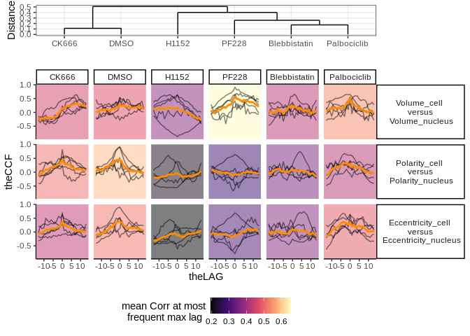
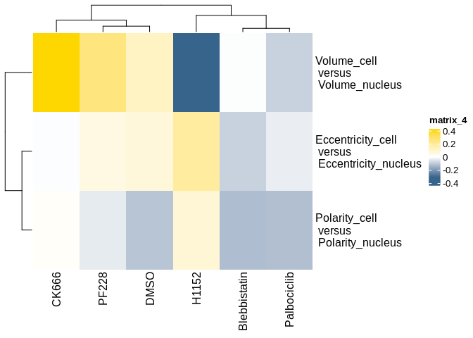
After running lts_in(), the output can be plotted with the three
lifeTimes plotting functions. Examples are below:
#View results
lts_plot_ccfs(lts_oneCat)lts_plot_ClustSum(lts_oneCat)
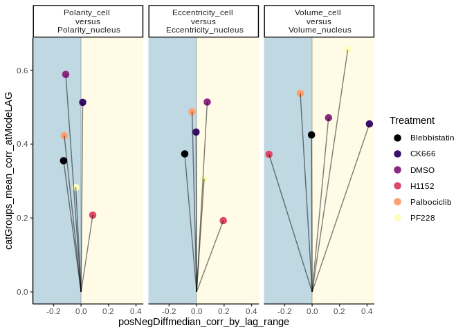
This example of lts_plot_coupled() shows two plots of the same data,
and how the colouring and faceting variables can be switched with the
.lts_colour_by = and `.lts_facet_by =``` parameters.
lts_plot_coupled(lts_oneCat,
                 .lts_colour_by = "cat1",
.lts_facet_by = "cat2")lts_plot_coupled(lts_oneCat,
.lts_colour_by = "cat2",
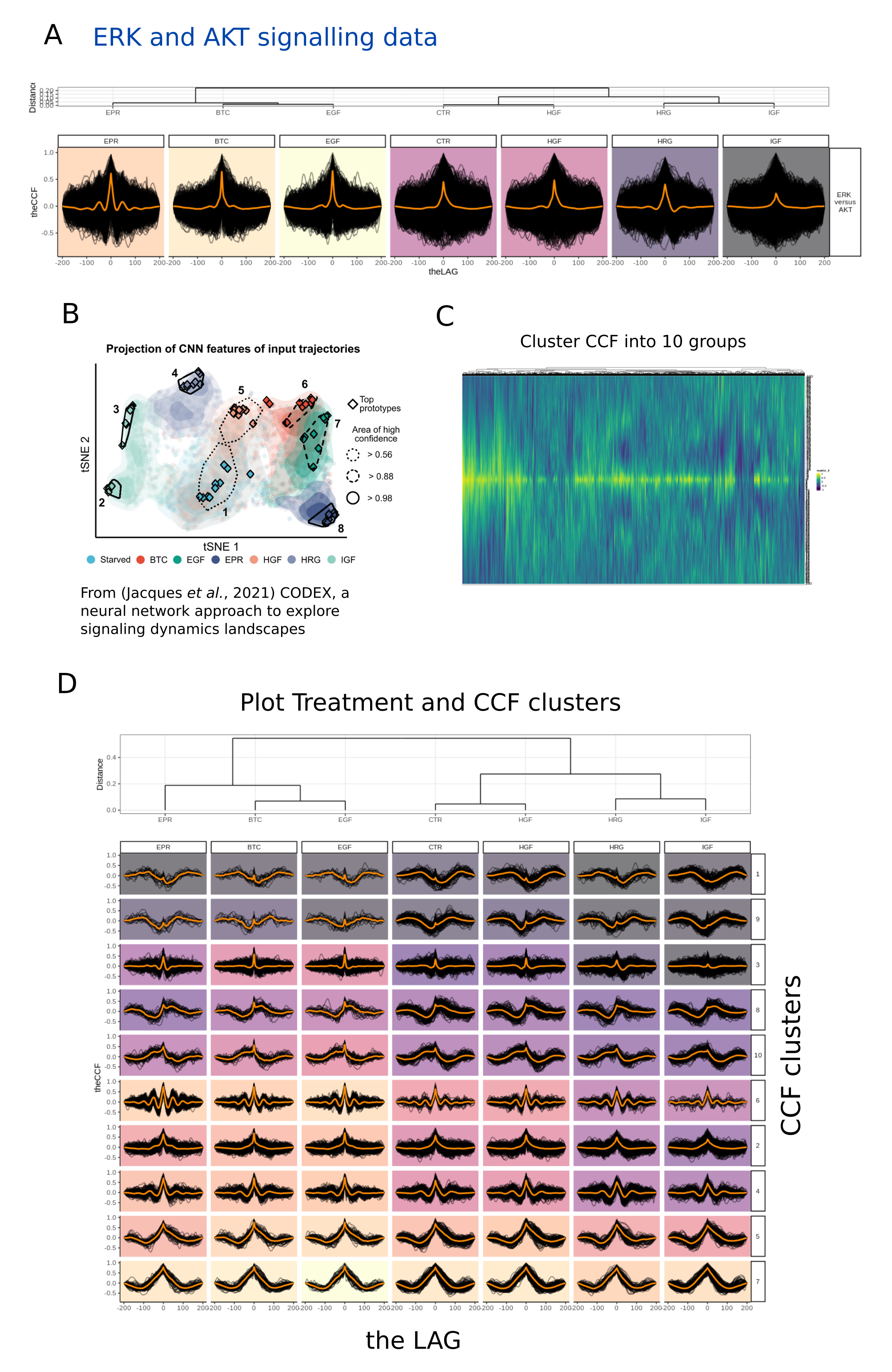
.lts_facet_by = "cat1")Data from Jacques et al., 2021
Decomposing the ERK (x) and AKT (y) cross-correlations foeach each
treatment,
results in clustering of treatments, broadly similar
to distribution in tSNE
space by neural networks (D). Each
treatment also has a different enrichment
for each cluster, for
example CTR (control) cells are enriched for
clusters 1, 9, and 7
relative to EGF, BTC, and EPR.
ERK and AKT data mining .
CCF from data measuring AKT and ERK activity following 7 different
treatments
(Jacques et al., 2021) (A), were visualised (B). Wide
variation in CCF indicated
subgroups may be present (B). CCFs
were clustered and labelled (C), and data
were plotted in
lifeTimes (D). Decomposition of each treatment into different
CCF
patterns, shows charactestic enrichment from different treatments (D).
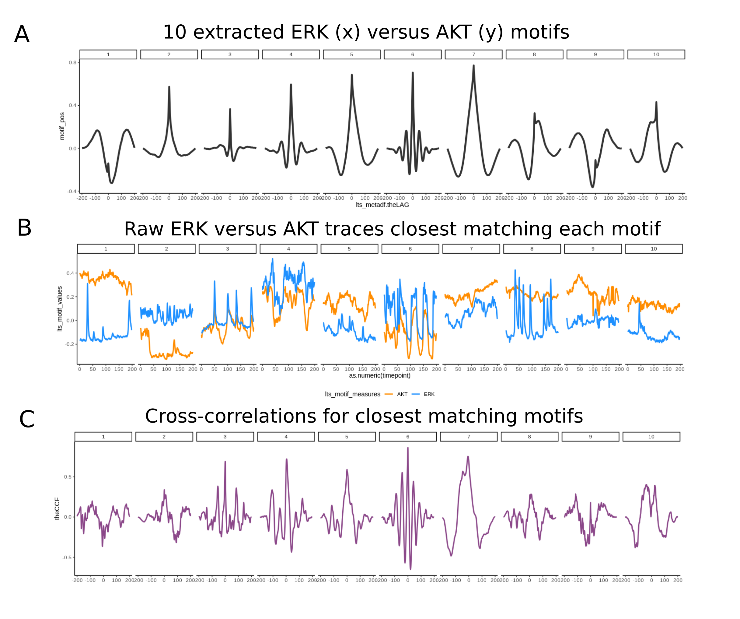
lifeTimes can be used to find motifs, or chacteristic relationships between
sets of variables. Here 10 motifs of ERK and AKT are shown.
CCF Motif Extraction .
Average traces for each of 10 CCF clusters identified in ERK versus AKT
traces
(data from Jacques et al., 2021). The raw traces most
closely matching each
motif (least sum of squared errors) (B).
The calculated cross-correlation for
each pair of raw traces (C).
Fin.
© 2022 GitHub, Inc. Terms Privacy Security Status
