Let’s take a look at the data!
# Read data

schengen_18 <- read_csv("2018-data-for-consulates.csv", guess_max = 2001)
## Parsed with column specification:
## cols(
## `Schengen State` = col_character(),
## `Country where consulate is located` = col_character(),
## Consulate = col_character(),
## `Airport transit visas (ATVs) applied for` = col_character(),
## `ATVs issued (including multiple)` = col_character(),
## `Multiple ATVs issued` = col_character(),
## `ATVs not issued` = col_character(),
## `Not issued rate for ATVs` = col_character(),
## `Uniform visas applied for` = col_character(),
## `Total uniform visas issued (including MEV)` = col_character(),
## `Multiple entry uniform visas (MEVs) issued` = col_character(),
## `Share of MEVs on total number of uniform visas issued` = col_character(),
## `Total LTVs issued` = col_character(),
## `Uniform visas not issued` = col_character(),
## `Not issued rate for uniform visas` = col_character(),
## `Total ATVs and uniform visas applied for` = col_character(),
## `Total ATVs and uniform visas issued (including multiple ATVs MEVs and LTVs)` = col_character(),
## `Total ATVs and uniform visas not issued` = col_character(),
## `Not issued rate for ATVs and uniform visas` = col_character()
## )
head(schengen_18)## # A tibble: 6 x 19
## `Schengen State` `Country where ~ Consulate `Airport transi~
## <chr> <chr> <chr> <chr>
## 1 Austria ALBANIA TIRANA <NA>
## 2 Austria ALGERIA ALGIERS <NA>
## 3 Austria ARGENTINA BUENOS A~ <NA>
## 4 Austria AUSTRALIA CANBERRA <NA>
## 5 Austria AZERBAIJAN BAKU 1
## 6 Austria BOSNIA AND HERZ~ SARAJEVO <NA>
## # ... with 15 more variables: `ATVs issued (including multiple)` <chr>,
## # `Multiple ATVs issued` <chr>, `ATVs not issued` <chr>, `Not issued
## # rate for ATVs` <chr>, `Uniform visas applied for` <chr>, `Total
## # uniform visas issued (including MEV)` <chr>, `Multiple entry uniform
## # visas (MEVs) issued` <chr>, `Share of MEVs on total number of uniform
## # visas issued` <chr>, `Total LTVs issued` <chr>, `Uniform visas not
## # issued` <chr>, `Not issued rate for uniform visas` <chr>, `Total ATVs
## # and uniform visas applied for` <chr>, `Total ATVs and uniform visas
## # issued (including multiple ATVs MEVs and LTVs)` <chr>, `Total ATVs and
## # uniform visas not issued` <chr>, `Not issued rate for ATVs and uniform
## # visas` <chr>
The different type of schengen visas given in the data are:
-
ATV (Airport transit visas): This type of visa is allows a person to travel through the internation zone of the schengen countries without entering the schengen area.
-
Uniform visa: This type of visa allows the holder to stay in the schengen area for a short amount of time. There are 3 types of uniform visas: single entry, double entry and Multiple Entry visa (MEV)
-
LTV (Limited Territorial Visa): This type of visa allows the holder to travel in only the schengen state that issued the visa.
Since most people will be interested in the uniform visas, we will only be exploring the uniform visa statistics from the data.
# Selecting useful columns
schengen_18 <- schengen_18 %>%
    select(`Schengen State`, `Country where consulate is located`, Consulate,
         `Uniform visas applied for`, `Total  uniform visas issued (including MEV)`,
         `Multiple entry uniform visas (MEVs) issued`, `Uniform visas not issued`)

schengen_18 <- schengen_18 %>%
  rename(schengen_state = `Schengen State`,
         consulate_country = `Country where consulate is located`,
         consulate = Consulate,
         applied = `Uniform visas applied for`,
         total_issued = `Total  uniform visas issued (including MEV)`,
         mev_issued = `Multiple entry uniform visas (MEVs) issued`,
         not_issued = `Uniform visas not issued`)
# Get missing states
schengen_18 %>%
filter(is.na(schengen_state))## # A tibble: 13 x 7
## schengen_state consulate_count~ consulate applied total_issued
## <chr> <chr> <chr> <chr> <chr>
## 1 <NA> <NA> <NA> <NA> <NA>
## 2 <NA> <NA> <NA> <NA> <NA>
## 3 <NA> <NA> <NA> <NA> <NA>
## 4 <NA> <NA> <NA> <NA> <NA>
## 5 <NA> <NA> Selectio~ 16,016~ 14,265,282
## 6 <NA> <NA> Total wo~ 16,016~ 14,265,282
## 7 <NA> <NA> Share of~ 100% 100%
## 8 <NA> <NA> <NA> <NA> <NA>
## 9 <NA> <NA> <NA> <NA> <NA>
## 10 <NA> <NA> <NA> <NA> <NA>
## 11 <NA> <NA> <NA> <NA> <NA>
## 12 <NA> <NA> <NA> <NA> <NA>
## 13 <NA> <NA> <NA> <NA> <NA>
## # ... with 2 more variables: mev_issued <chr>, not_issued <chr>
There are several rows with NA schengen state, They contain the summary statistics for the data. We do not need that row.
#Remove rows with NA state
schengen_18 <- schengen_18 %>%
filter(!is.na(schengen_state))#Convert columns to numeric
schengen_18 <- schengen_18 %>%
transform(applied = as.numeric(sub(",", "", applied)),
total_issued = as.numeric(sub(",", "", total_issued)),
mev_issued = as.numeric(sub(",", "", mev_issued)),
not_issued = as.numeric(sub(",", "", not_issued)))#Map data
states <- str_to_upper(unique(schengen_18$schengen_state))
world_map <- map_data(map = "world", region = "(?!ANTARCTICA)") %>%
mutate(region = str_to_upper(region))
#Some countries in the map data appear different than ones in our schengen data
world_map <- world_map %>%
mutate(region = recode(region,
`DEMOCRATIC REPUBLIC OF THE CONGO` = "CONGO (DEMOCRATIC REPUBLIC)",
`REPUBLIC OF CONGO` = "CONGO (BRAZZAVILLE)",
`PALESTINE` = "PALESTINIAN AUTHORITY",
`RUSSIA` = "RUSSIAN FEDERATION",
`IVORY COAST` = "COTE D'IVOIRE",
`UK` = "UNITED KINGDOM",
`MACEDONIA` = "NORTH MACEDONIA",
`TRINIDAD` = "TRINIDAD AND TOBAGO",
`TOBAGO` = "TRINIDAD AND TOBAGO"))#Applications per country
schengen_18 %>%
group_by(consulate_country) %>%
summarise(applications = sum(applied, na.rm = T)) %>%
right_join(., world_map, by = c("consulate_country" = "region")) %>%
ggplot() +
geom_map(map = world_map, mapping = aes(map_id = consulate_country, fill = applications)) +
expand_limits(x = world_map$long, y = world_map$lat) +
scale_fill_distiller(palette = 1, direction = 1,
breaks = c(1000000, 2000000, 3000000),
labels = c("1 Million", "2 Million", "3 Million")) +
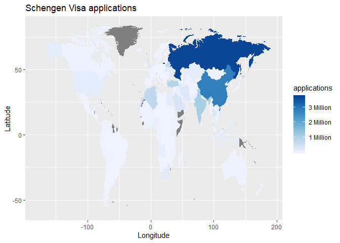
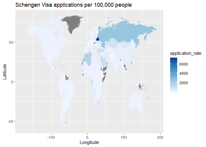
labs(x = "Longitude", y = "Latitude", title = "Schengen Visa applications")Majority of applications are from Russia (3.69 Million), China (2.82 Million) and India (1.08 Million). We can expect a higher number of visa applications from countries with higher population. We can normalize this data by country population in 2018 data from world bank to get the visa application rate per 100,000 people.
#Application rate per country
population_18 <- read_csv("2018-population.csv")
## Parsed with column specification:
## cols(
## `Country Name` = col_character(),
## `Country Code` = col_character(),
## `Series Name` = col_character(),
## `Series Code` = col_character(),
## `2018 [YR2018]` = col_character()
## )
# Transforming population data into a format similar to other data
population_18 <- population_18 %>%
  select(`Country Name`, `2018 [YR2018]`) %>%
  rename(country = `Country Name`, population = `2018 [YR2018]`) %>%
  transform(country = str_to_upper(country),
            population = as.numeric(population)) %>%
  mutate(country = recode(country,
                          `CONGO, DEM. REP.` = "CONGO (DEMOCRATIC REPUBLIC)",
                          `CONGO, REP.` = "CONGO (BRAZZAVILLE)",
                          `UNITED STATES` = "USA",
                          `VENEZUELA, RB` = "VENEZUELA",
                          `IRAN, ISLAMIC REP.` = "IRAN",
                          `EGYPT, ARAB REP.` = "EGYPT",
                          `SYRIAN ARAB REPUBLIC` = "SYRIA",
                          `KYRGYZ REPUBLIC` = "KYRGYZSTAN",
                          `KOREA, REP.` = "SOUTH KOREA",
                          `KOREA, DEM. PEOPLE’S REP.` = "NORTH KOREA"))
## Warning in eval(substitute(list(...)), `_data`, parent.frame()): NAs
## introduced by coercion
#Keeping only those countries that we need
population_18 <- population_18 %>%
  semi_join(schengen_18, by = c("country" = "consulate_country"))

schengen_18 %>%
  group_by(consulate_country) %>%
  summarise(applications = sum(applied, na.rm = T)) %>%
  left_join(population_18, by = c("consulate_country" = "country")) %>%
  mutate(application_rate = 100000 * applications/population) %>%
  right_join(., world_map, by = c("consulate_country" = "region")) %>%
  ggplot() +
  geom_map(map = world_map, mapping = aes(map_id = consulate_country, fill = application_rate)) +
  expand_limits(x = world_map$long, y = world_map$lat) +
  scale_fill_distiller(palette = 1, direction = 1) +
  labs(x = "Longitude", y = "Latitude",
title = "Schengen Visa applications per 100,000 people")#Application rate by population
schengen_18 %>%
group_by(consulate_country) %>%
summarise(applications = sum(applied, na.rm = T)) %>%
left_join(population_18, by = c("consulate_country" = "country")) %>%
mutate(application_rate = 100000 * applications/population) %>%
top_n(20, application_rate) %>%
ggplot(mapping = aes(x = reorder(consulate_country, application_rate),
y = application_rate)) +
geom_point(col = "red") +
geom_segment(aes(x = consulate_country, xend = consulate_country,
y = 0, yend = application_rate)) +
coord_flip() +
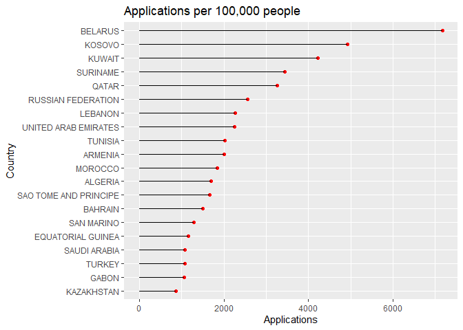
labs(x = "Country", y = "Applications", title = "Applications per 100,000 people")We can see that countries with smaller population like Belarus, Kosovo, Kuwait, Russia have a higher visa application rate per 100,000 people. But Russia is still at the 6th position. A lot of people from Russia apply for schengen visas!
#Consuates per country
schengen_18 %>%
  group_by(consulate_country) %>%
  summarise(n_consulates = n()) %>%
  top_n(20, n_consulates) %>%
  ggplot(aes(x = reorder(consulate_country, n_consulates), y = n_consulates)) +
  geom_point(col = "red") +
  geom_segment(aes(x = consulate_country, xend = consulate_country,
                   y = 0, yend = n_consulates)) +
  coord_flip() +
  labs(x = "Country", y = "Number of consulates",
       title = "Number of consulates per country")
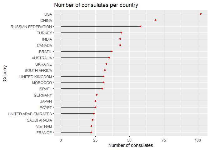
Most number of consulates are in USA, China and Russia. Let us look at the countries with highest application rate per consulate.
#Average application rate per consulate
schengen_18 %>%
  group_by(consulate_country) %>%
  summarise(applications_per_consulate = sum(applied)/n()) %>%
  top_n(20, applications_per_consulate) %>%
  ggplot(aes(x = reorder(consulate_country, applications_per_consulate),
             y = applications_per_consulate)) +
  geom_point(col = "red") +
  geom_segment(aes(x = consulate_country, xend = consulate_country,
                   y = 0, yend = applications_per_consulate)) +
  coord_flip() +
  labs(x = "Country", y = "Applications per consulate",
       title = "Average applications per consulate")
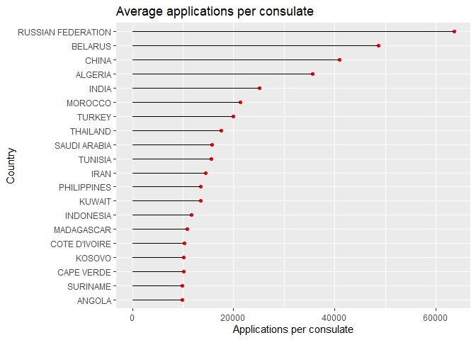
Russia, Belarus, China, Argentina, India and Morocco recieve the most number of applications per consulate.
#State with most issued visas
schengen_18 %>%
  group_by(schengen_state) %>%
  summarize(issued = sum(total_issued, na.rm = T), mev = sum(mev_issued, na.rm = T)) %>%
  top_n(20, issued) %>%
  ggplot(aes(x = reorder(schengen_state, issued))) +
  geom_col(aes(y = issued, fill = 'lightblue'), alpha = 0.8, color = 'lightblue4') +
  geom_col(aes(y = mev, fill = 'pink'), alpha = 0.3, color = 'red') +
  coord_flip() +
  scale_fill_identity(name = "Color", guide = "legend",
                      labels = c("Total Uniform visas", "MEVs share")) +
  labs(x = "Schengen State", y = "Total visas issued",
       title = "Schengen state that issues most uniform visas in 2018") +
  scale_y_continuous(breaks = c(1e+06, 2e+06, 3e+06),
                     labels = c("1 Million", "2 Million", "3 Million"))
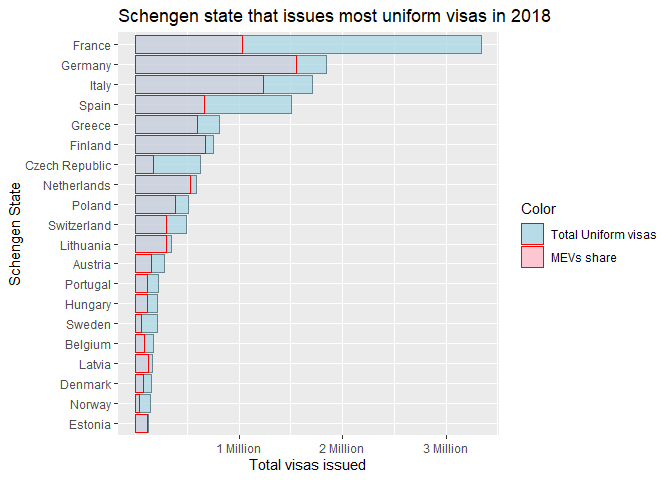
France issued nearly 3.35 Million visas in 2018, nearly twice as much as Germany that comes at the 2nd place with nearly 1.84 Million visas issued. However the share of MEVs issued in France is far less. France, Germany, Italy and Spain issued more than 1 Million visas in 2018. Germany issued the most MEVs followed by Italy in 2018. For countries like Finland, Netherlands and Estonis, most of the Uniform visas issued were MEVs.
#Countries that got most visas
schengen_18 %>%
group_by(consulate_country) %>%
summarise(issued = sum(total_issued, na.rm = T), mev = sum(mev_issued, na.rm = T)) %>%
top_n(20, issued) %>%
ggplot(aes(x = reorder(consulate_country, issued))) +
geom_col(aes(y = issued, fill = 'lightblue'), alpha = 0.8, color = 'lightblue4') +
geom_col(aes(y = mev, fill = 'pink'), alpha = 0.3, color = 'red') +
coord_flip() +
scale_fill_identity(name = "Color", guide = "legend",
labels = c("Total Uniform visas", "MEVs issued")) +
labs(x = "Country", y = "Total visas issued",
title = "Consulate Countries where most visas were issued") +
scale_y_continuous(breaks = c(1e+06, 2e+06, 3e+06),
labels = c("1M", "2M", "3M"))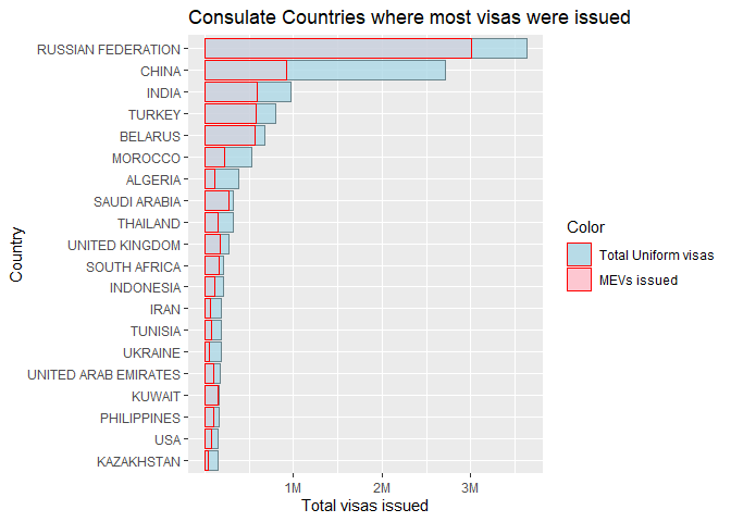 Russia and China tops the list with 3.64 Million and 2.7 Million visa
issuances respectively. After Russia and China, there is a huge drop in
visa issuance rate. India comes 3rd with 0.97 Million visas issued,
which is almost one-third of China’s visa issuances in 2018. Majority of
visas issued in China are not MEVs. For countries like Saudi Arabia,
South Africa and Kuwait, almost all of the uniform visas issued in 2018
were MEVs.
#Visa issuances by population
schengen_18 %>%
  group_by(consulate_country) %>%
  summarise(issued = sum(total_issued, na.rm = T), mev = sum(mev_issued, na.rm = T)) %>%
  left_join(population_18, by = c("consulate_country" = "country")) %>%
  mutate(issuance_rate = 100000*issued/population, mev_rate = 100000*mev/population) %>%
  top_n(20, issuance_rate) %>%
  ggplot(aes(x = reorder(consulate_country, issuance_rate))) +
  geom_col(aes(y = issuance_rate, fill = 'lightblue'), alpha = 0.8, color = 'lightblue4') +
  geom_col(aes(y = mev_rate, fill = 'pink'), alpha = 0.3, color = 'red') +
  coord_flip() +
  scale_fill_identity(name = "Color", guide = "legend",
                      labels = c("Total Uniform visas", "MEVs issued")) +
  labs(x = "Country", y = "Visas issued",
       title = "Consulate countries with the highest visas issued per 100k people")
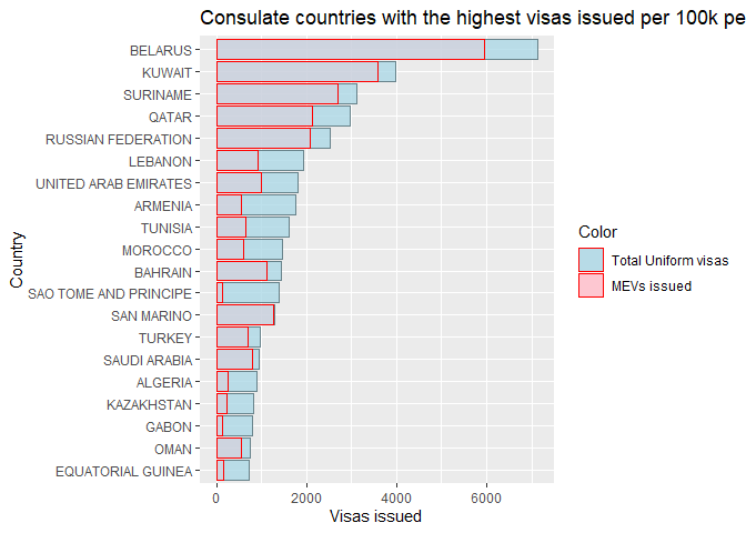
Smaller countries like Belarus, Kuwait, Suriname and Qatar have the highest visa issuance rate per 100,000 people. Most of these countires have a very good share of MEV issuance.
