hockeyR

This package contains various functions to scrape and clean play-by-play data from NHL.com. Season play-by-play data scraped with these functions can be found in the hockeyR-data repository. It also contains functions to scrape data from hockey-reference.com, including standings, player stats, and jersey number history.

Installation

Before installing, confirm that your version of R is updated to at least 4.1.0. This will ensure R can handle R’s native pipe operator |>, which was unavailable until 4.1.0. If you do not wish to update to R 4.1.0, can install the development version from GitHub instead.

If you don’t know which version of R is installed, try verson$version.string in your R console.

version$version.string
#> [1] "R version 4.1.0 (2021-05-18)"

Install the released version of hockeyR (requires R 4.1.0) from CRAN with:

install.packages("hockeyR")

Install the development version of hockeyR (requires R 3.5) from GitHub with:

# install.packages("devtools")
devtools::install_github("danmorse314/hockeyR")

Usage

Load the package (and any others you might need—for plotting an ice surface I highly recommend the sportyR package).

library(hockeyR)
library(tidyverse)
library(sportyR)

Loading season play-by-play

The fastest way to load a season’s play-by-play data is through the load_pbp() function, which pulls the desired season(s) from hockeyR-data. load_pbp() also has the advantage of accepting more explicit values for the seasons desired. For example, if you want to get the play-by-play for the 2020-2021 NHL season, all of load_pbp('2020-2021'), load_pbp('2020-21'), and load_pbp(2021) will get it for you.

pbp <- load_pbp('2018-19')

The available data goes back to the 2010-2011 season as of now, as the NHL JSON source used for this scraper doesn’t include detailed play-by-play prior to that.

All variables available in the raw play-by-play data are included, along with a few extras added on including:

shot_distance
shot_angle
x_fixed
y_fixed

The shot_distance and shot_angle are measured in feet and degrees, respectively. The variables x_fixed and y_fixed are transformations of the x and y event coordinates such that the home team is always shooting to the right and the away team is always shooting to the left. For full details on the included variables, see the scrape_game() documentation.

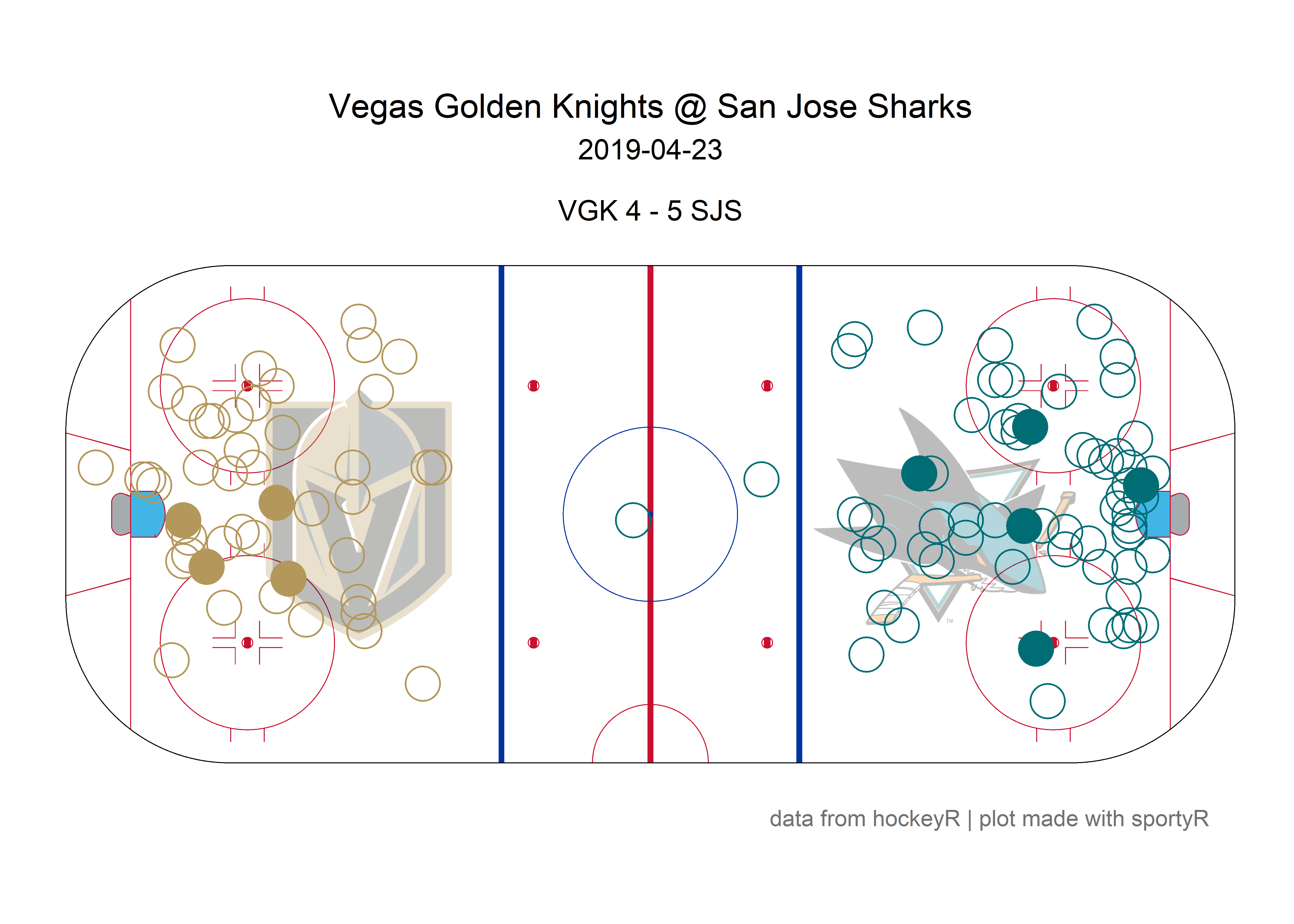
As mentioned above, an easy way to create a shot plot is through the sportyR package. You can also use the included team_colors_logos data to add color and team logos to your plots.

# get single game
game <- pbp %>%
  filter(game_date == "2019-04-23" & home_abbreviation == "SJS")

# grab team logos & colors
team_logos <- hockeyR::team_logos_colors %>%
  filter(team_abbr == unique(game$home_abbreviation) | team_abbr == unique(game$away_abbreviation)) %>%
  # add in dummy variables to put logos on the ice
  mutate(x = ifelse(full_team_name == unique(game$home_name), 50, -50),
         y = 0)

# add transparency to logo
transparent <- function(img) {
  magick::image_fx(img, expression = "0.3*a", channel = "alpha")
}

# get only shot events
fenwick_events <- c("MISSED_SHOT","SHOT","GOAL")

shots <- game %>% filter(event_type %in% fenwick_events) %>%
  # adding team colors
  left_join(team_logos, by = c("event_team_abbr" = "team_abbr"))

# create shot plot
geom_hockey("nhl") +
  ggimage::geom_image(
    data = team_logos,
    aes(x = x, y = y, image = team_logo_espn),
    image_fun = transparent, size = 0.22, asp = 2.35
    ) +
  geom_point(
    data = shots,
    aes(x_fixed, y_fixed),
    size = 6,
    color = shots$team_color1,
    shape = ifelse(shots$event_type == "GOAL", 19, 1)
    ) +
  labs(
    title = glue::glue("{unique(game$away_name)} @ {unique(game$home_name)}"),
    subtitle = glue::glue(
    "{unique(game$game_date)}\n
    {unique(shots$away_abbreviation)} {unique(shots$away_final)} - {unique(shots$home_final)} {unique(shots$home_abbreviation)}"
    ),
    caption = "data from hockeyR | plot made with sportyR"
    ) +
  theme(
    plot.title = element_text(hjust = 0.5),
    plot.subtitle = element_text(hjust = 0.5),
    plot.caption = element_text(hjust = .9)
    )

Future Work

Getting clean data for games going back to the start of the NHL RTSS era (2007-2008 season) is in the works. There are also plans to create a basic expected goals model and perhaps a win probability model that would include xG values for each shot and win probabilities for each play, similar to the expected points model found in the nflfastR package. And of course, scraping the upcoming NHL season and updating the data daily is planned for the 2021-2022 season.

Acknowledgments

Everyone involved in making the nflverse, the premier data source for NFL stats that inspired this whole project
The Evolving Wild twins, whose old NHL scraper helped enormously in getting player on-ice data joined to the raw play-by-play data in here.
Tan Ho, whose twitch streams on web scraping and JSON wrangling quite literally took me from 0 web scraping knowledge to building this package

skent259 / hockeyR