heagy-2018-dc-casing

Overview

These notebooks were used to perform the analysis and generate the figures shown "Direct current resistivity with steel-cased wells" by Lindsey Heagy and Doug Oldenburg published in Geophysical Journal International, as well as that shown in Chapter 4 of the thesis Electromagnetic imaging of subsurface injections.

We examine the use of DC resistivity for detecting flaws in a well in a casing integrity experiment, and examine factors influencing our ability to excite and detect a target at depth.

Citation

Heagy, L. J., & Oldenburg, D. W. (2018). Direct current resistivity with steel-cased wells. Geophysical Journal International.

@article{10.1093/gji/ggz281,
    author = {Heagy, Lindsey J and Oldenburg, Douglas W},
    title = "{Direct current resistivity with steel-cased wells}",
    journal = {Geophysical Journal International},
    year = {2019},
    month = {06},
    issn = {0956-540X},
    doi = {10.1093/gji/ggz281},
    url = {https://doi.org/10.1093/gji/ggz281},
    eprint = {http://oup.prod.sis.lan/gji/advance-article-pdf/doi/10.1093/gji/ggz281/28836831/ggz281.pdf},
}

1_DC_Flawed_Steel_Cased_Wells.ipynb
- examines the feasibility of using DC resistivity for detecting a flaw in a steel-cased well and investigates the impact of parameters such as the background conductivity on our ability to detect a flaw from data collected at the surface.
- This notebook was used to produce:
  - Figures 1, 2, 4, 5, 6, 9, 10, 11 in Heagy & Oldenburg (2018)
  - Figures 4.1, 4.2, 4.4, 4.5, 4.6, 4.9, 4.10 and 4.11 in the thesis
2_DC_Flawed_Steel_Cased_Wells_Short_well.ipynb
- looks at hte impact of the vertical extent of the flaw on the distribution of charges.
- Used to produce:
  - Figure 3 in Heagy & Oldenburg (2018)
  - Figure 4.3 in the thesis
3_DC_Flawed_Steel_Cased_Wells_layer
- looks at the impact of a conductive or resistive layer on our ability to detect a flaw.
- Used to create:
  - Figures 7, 8 in Heagy & Oldenburg (2018)
  - Figures 4.7 and 4.8 in the thesis
4_DC_source_location.ipynb
- looks at the impact of the source electrode location on our ability to deliver current to depth.
- This was used to produce:
  - Figures 12, 13 in Heagy & Oldenburg (2018)
  - Figures 4.12 and 4.13 in the thesis
5_DC_target.ipynb
- Examines our ability to excite a conductive or resistive target at depth, looks at the impact of having an electrical connection (or not) between the target and the casing
- This notebook was used to produce:
  - Tables 1, 2 and Figures 14, 15, 16, 17, 18 in Heagy & Oldenburg (2018)
  - Tables 4.1, 4.2 and Figures 4.14, 4.15, 4.16, 4.17, 4.18 in the thesis
6_DC_target_3D_cartesian.ipynb
- here, we use a born approximation approach to examine our ability to excite a target offset from the well.
- This notebook was used to produce:
  - Figures 19, 20, 21 in Heagy & Oldenburg (2018)
  - Figures 4.19, 4.20, 4.21 in the thesis
7_DC_Approximating_Steel_Cased_Wells.ipynb
- This notebook looks at approximations of a steel cased well by a solid cylinder, either with a conductivity equal to steel, or a conductivity that preserves the cross-sectional conductance of the well.
- This notebook was used to produce:
  - Figures 22, 23 in Heagy & Oldenburg (2018)
  - Figures 4.22, 4.23 in the thesis
8_DC_Approximating_Steel_Cased_Wells_layered_background.ipynb
- Similar to notebook 7, this notebook looks at approximations to the steel cased well by a solid cylinder in a layered background.
- It was used to produce:
  - Figures 24, 25 in Heagy & Oldenburg (2018)
  - Figures 4.24, 4.25 in the thesis
9_DC_Approximating_Steel_Cased_Wells_Cartesian.ipynb
- This notbook looks at approximations of the steel cased well onto a cartesian mesh.
- This notebook was used to create:
  - Figure 26 in Heagy & Oldenburg (2018)
  - Figures 4.26 in the thesis

Launching the notebooks

Online

The notebooks can be run online through mybinder or azure notebooks.

Locally

To run them locally, you will need to have python installed, preferably through anaconda.

You can then clone this repository. From a command line, run

git clone https://github.com/simpeg-research/heagy-2018-dc-casing.git

Then cd into the heagy-2018-dc-casing

cd heagy-2018-dc-casing

To setup your software environment, we recommend you use the provided conda environment

conda env create -f environment.yml
source activate dc-casing-environment

alternatively, you can install dependencies through pypi

pip install -r requirements.txt

You can then launch Jupyter

jupyter notebook

Jupyter will then launch in your web-browser.

Running the notebooks

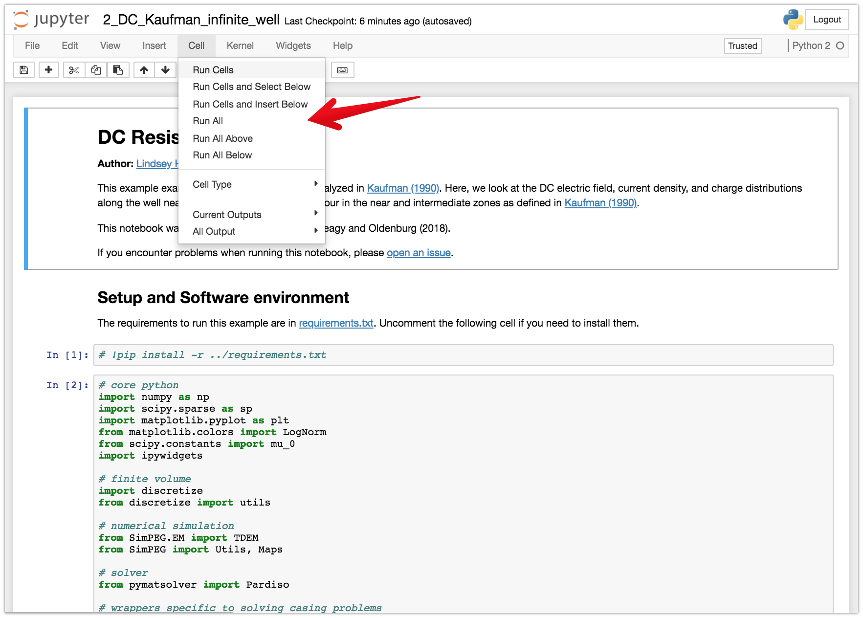
Each cell of code can be run with shift + enter or you can run the entire notebook by selecting cell, Run All in the toolbar.

For more information on running Jupyter notebooks, see the Jupyter Documentation

Issues

If you run into problems or bugs, please let us know by creating an issue in this repository.

License

These notebooks are licensed under the MIT License which allows academic and commercial re-use and adaptation of this work.

Version

Current version: 0.0.3

simpeg-research / heagy-2018-dc-casing