This project was originally made for UC Berkeley's EE122: Introduction to Communication Networks (Spring 2023).
Team: Sidharth Rajaram, Pranav Eranki, Sasha Sato, Nithila Poongovan
Introduction
In order to better understand the performance considerations and requirements of LEO internet satellite constellations, we built a simulated model of the Starlink network, complete with real orbital data, ground stations, packet routing, and metrics generation. Specifically, we wanted to investigate how network performance (measured by packets dropped, downtime, and satellite utilization) changed with respect to the size of the LEO constellation (number of satellites).
Our simulation consists of three main components. First, the network topology, which comprises the programmatic representations of Starlink satellites, ground stations, ground nodes (end users) and the geographic environment. Next, simulated traffic and routing, which are defined by the process of routing packets from one end user to ground stations or other end users (and how they are affected by link capacity / range and satellite movement). The final component was metrics generation; we decided to measure the number of packets dropped, downtime of packet transmission (how often ground nodes were unable to connect to the satellites), and the overall number of satellites utilized by the routing algorithm during the entire simulation.
Realism
The satellite constellation’s operation is realistically simulated with the aid of open-source Python libraries poliastro (interactive astrodynamics, orbital mechanics, and visualizations), SGP4 (satellite trajectory algorithm), and astropy (astronomical coordinate system), with an update to the positions of the satellites being done at the end of every timestep of the routing algorithm. NetworkX is also used for graphing. In order to make our simulation as realistic as possible, we supplied our code with real orbital tracking data (in the form of general perturbations data) published by the US government’s North American Aerospace Defense Command (NORAD) space tracking system.
Implementation / Object Representations
We created an object-oriented representation of the network topology by defining the InternetSatellite, Simulator, GroundNode, and Packet classes. An InternetSatellite instance primarily represents a single Starlink satellite’s physical state (ephemeris, orbital step), motion over time, and ultimately, a satellite node in the overall network topology. We initialized each InternetSatellite instance to correspond with a real Starlink satellite, complete with the real ID and ephemeris of that Starlink satellite. With the real ephemeris for each Starlink satellite, we used SGP4 and the poliastro library’s OrbitPlotter function to visualize the entire constellation’s path. The below example shows a 100-satellite Starlink constellation’s orbital paths around Earth (the overlapping colors are due to the fact that SpaceX positions rows of satellites offset on the exact same orbital path):

GroundNode instances can be of two types: a ground terminal or a ground station. Ground terminals represent end users who are trying to connect to the internet; ground terminals are our “normal” nodes, which try to connect with the internet satellites. Ground stations represent the gateway for the Starlink satellites to connect to the internet. There are three types of routing—terminal to satellite, satellite to satellite, and satellite to station. GroundNodes are represented by their node_type and positional data.
One significant challenge in our simulation was creating a cohesive coordinate system for all nodes in our network from which we could derive accurate distance data. Using astropy, we were able to convert the latitude/longitude coordinates of static locations of ground nodes to 3D coordinates (based on a geocentric point of reference). Similarly, we were able to use poliastro and ephemeris data of the Starlink satellites to produce their coordinates in the same 3D coordinate basis as the ground locations. With all network nodes represented in the same coordinate system, we could easily calculate inter-node distance, which was crucial for the creation of our network graph and our routing algorithm.
Provided with lists of satellite objects, ground terminal objects, and ground station objects, a Simulator instance uses NetworkX to construct a graph using the aforementioned objects as wrappers for nodes in the graph. With undirected edges, all satellites are fully connected amongst themselves, all satellite nodes are connected to ground stations, and all ground terminals are connected to all satellites. Note that, in this regard, “connected” just means there exists an edge in the graph definition; it doesn’t guarantee internet connectivity during the simulation. In the actual simulation, a node on the ground and a satellite in orbit are considered out of range if they are further than a pre-calculated Euclidean distance threshold. Based on publicly available Starlink specifications, we calculated this value to be around 1404 km (Pekhterev). However, for our own curiosity we kept this value as a modifiable hyperparameter, which could be useful for testing the performance of different models of satellites or orbit parameters.
The edges are initialized with costs and capacities. The cost is defined as the Euclidean distance between two nodes. The capacity for an edge is sampled from a normal probability distribution with mean 20 Mbps and standard deviation 1 Mbps. This is based on average statistics of Starlink performance right now (Pekhterev).

Simulated Packet Flow
After creating the graph of the simulated network topology, we inject a stream of n Packet objects, each initialized with a source node ID, destination node ID, and size. Our simulator instance also facilitates the dynamic properties of our simulation, ensuring that the satellites’ orbital positions and packet “locations” update accordingly with each time step.
In our simulation, each Packet object originates from a ground terminal and is destined for a ground station (in order to connect to the wider Internet). As mentioned earlier, there are three distinct stages for routing a single packet: (1) packet to satellite, (2) satellite to satellite, and (3) satellite to ground station. In the first stage, a packet is transmitted to the closest in-range satellite; this greedy selection represents the predominant first-come, first-serve paradigm of connectivity. If there are no satellites within range, the packet remains in a queue at the ground terminal (this means downtime for the end user since they cannot transmit their packet). Once the packet is received by a satellite, the shortest path to the ground station, given the remaining capacities of links between satellites, is calculated. This reflects our implementation of FHRP (more on this below). Once the path is calculated, the path is naively obeyed with each edge being traversed in a timestep. When a packet is “transmitted” across an edge during its path, that packet’s size is subtracted from the edge’s capacity. If an edge on a packet’s path has zero present capacity, the packet is forced to wait in a queue. If a packet remains in a queue (either on a satellite or on a ground node) for too long, it is declared stale and dropped from the flow entirely.
At its core, FHRP makes use of the footprints of the satellites in the initial route as the reference for re-routing (Uzunalioglu). This has a tradeoff—getting orbital data and doing large-scale path updates at every step is very costly, but sending data to a congested, out-of-range, or possibly inactive link could be costly for valuable time and bandwidth, especially as acks arrive slowly due to long distances. There could also be a marginally faster path based on predictively seeing where satellites will be 100ms or so in the future; however, these marginally faster paths are not considered due to FHRP’s reliance on the initial state, or “footprint”, of satellite positions.
Using the Simulator instance and the stream of Packet objects, we were able to generate simulated metrics for constellation and network performance. First, we were able to measure the number of packets that were dropped. Second, we created a novel metric based on our measurement of the total waiting time of packets called the Downtime Percentage and calculated as (time steps spent waiting by all packets) / (total time steps * total number of packets). This metric was our way of capturing the availability of the network, since a greater Downtime Percentage meant that packets spent a lot more time waiting at nodes, whether that be on the ground or on satellites. Another metric we measured was the number of intra-satellite hops, which we used to represent how the constellation was utilized.
Simulation and Analysis
In order to address our original questions about satellite internet performance, we wanted to see how the performance characteristics of the network are affected by the LEO constellation’s size, i.e., the number of satellites. We initialized a simulated environment of 3 ground terminals, 1 ground station, and n Starlink satellites (where n=25, 50, 100). Sticking to our initial curiosity about Starlink performance in Ukraine, we decided to position ground terminals in points of interest in Ukraine (Kyiv Airport, a hospital in Kyiv, Odessa Airport, and a rural hospital in the middle of the country). We placed the ground station north of Kyiv. We simulated a flow of 10 packets from these ground terminals with 25, 50, and 100 Starlink satellites and produced the aforementioned metrics.
Below is an example of a simulation using 100 randomly picked Starlink satellites with 10 randomly generated packets being transmitted from the aforementioned ground terminals in Ukraine. We begin with the initial step for all the packets being determined using current data, leading them to move to the closest satellite, which subsequently begins their routing calculations. Some of the packets are able to make it to their destination on the first try (e.g., Packet 61057…), but others have issues with link capacity constraints, lack of service, and range, forcing them to either wait at a satellite or be routed to another satellite and so on.
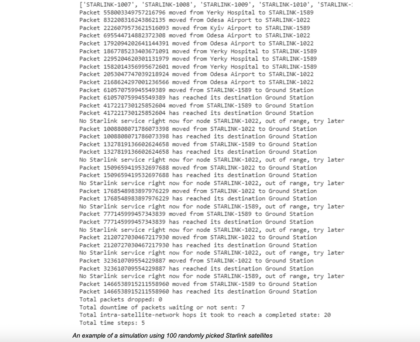
In this particular simulation, seven time steps were spent waiting at nodes across all packets. Since there were five total time steps and 10 total packets, this means the Downtime% was 7 / 50 = 14%. In this particular simulation, no packets were dropped, which means all packets were able to ultimately get to their destination, although some of the time some were waiting at nodes.
Simulation Results and Findings
Here are the average results we got across our trials of 25, 50, and 100 satellites:
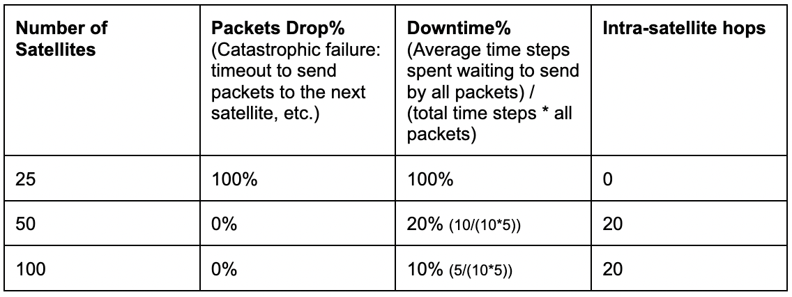
Performance (both the number of packets successfully sent and the downtime) improves with the number of satellites in the LEO constellation. However, packet drop rates and downtime are affected differently. We thought it was particularly interesting how downtime% decreased at a reduced rate when the constellation size was doubled from 50 to 100 versus when it was doubled from 25 to 50. These numbers are consistent with an exponential decrease in downtime as the number of satellites increases. We believe this is due to the unavoidable constraints of link capacity to a single satellite, because even with 100 satellites, there were still only 1-2 satellites serving the Ukraine region (note the same two satellites STARLINK-1589 and STARLINK-1022 used in all the packets’ first hop in the simulation output in the previous section). This would explain why the largest LEO internet satellite constellation providers are focusing on using sheer numbers to overcome these diminishing service quality improvements (e.g., Starlink’s fleet size is 3800 with an eventual goal of 42,000 satellites).