si-the-pie / pct

Development of a 'Propensity to Cycle Tool'

pct: Propensity to cycle tool

This repository allows users to estimate the 'propensity to cycle' between different origin-destination pairs.

The project is funded by the Department for Transport (DfT) so the initial case studies will be taken from the UK. However, it is expected that the methods will be of use elsewhere. For that reason, attempts have been made to make the examples generalisable. All examples presented here are reproducible using code in this repository and data stored in the pct-data repository.

If you run the following lines of code on from a local copy of the pct repository you will get the same results.

A simple example

source("set-up.R")
# load some flow data
fleeds <- read.csv("README_files/data/sample-leeds-centre-dists.csv")
# load the zones
leeds <- readOGR("README_files/data", "leeds-central-sample")

## OGR data source with driver: ESRI Shapefile 
## Source: "README_files/data", layer: "leeds-central-sample"
## with 25 features
## It has 3 fields

Now we can estimate propensity to cycle, by using the distance decay function from (Iacono et al. 2010):

$$ p = \alpha e^{- \beta d} $$

where $\alpha$, the proportion of made for the shortest distances and $\beta$, the rate of decay are parameters to be calculated from empirical evidence.

To implement this understanding in R code we can use the following function:

# Distance-dependent mode switch probs
iac <- function(x, a = 0.3, b = 0.2){
  a * exp(-b * x)
}

Apply this function to openly accessible flow data:

fleeds$p_cycle <- iac(fleeds$dist / 1000)
fleeds$n_cycle <- fleeds$p_cycle * fleeds$All.categories..Method.of.travel.to.work
fleeds$pc1 <- fleeds$n_cycle - fleeds$Bicycle

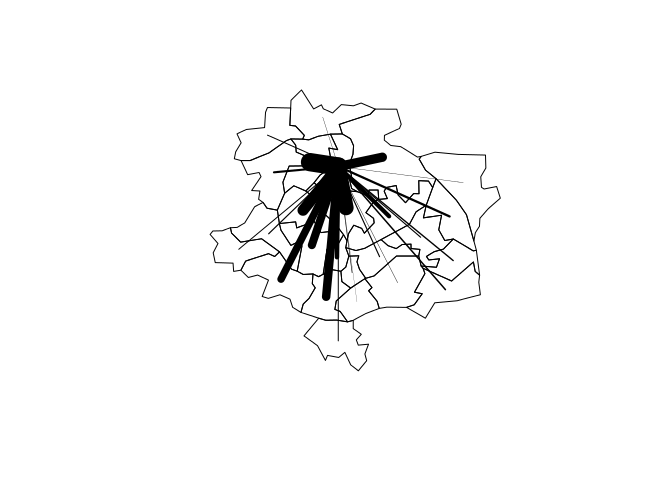
Now we can create a simple visualisation of the result:

plot(leeds)

for(i in which(fleeds$Area.of.residence == leeds$geo_code[1])){
  from <- leeds$geo_code %in% fleeds$Area.of.residence[i]
  to <- leeds$geo_code %in% fleeds$Area.of.workplace[i]
  x <- coordinates(leeds[from, ])
  y <- coordinates(leeds[to, ])
  lines(c(x[1], y[1]), c(x[2], y[2]), lwd = fleeds$pc1[i] )
}

Set the CS_API_KEY Environment variable

Some of the examples pull data from the CycleStreets.net API. Once you have a token, you can add it in Ubuntu as a session variable using the following in your terminal

echo "export CS_API_KEY='my_token'" >> ~/.profile

or system wide variable

sudo echo "export CS_API_KEY='my_token'" > /etc/profile.d/cyclestreet.sh

Set up rgdal

The version of gdal needs to be newer than 1.11

rgdal::getGDALVersionInfo()

## [1] "GDAL 1.11.2, released 2015/02/10"

# Should return GDAL 1.11.2, released 2015/02/10 (or newer)

It is possible to use the following Personal Package Archive (PPA) to get the latest version of gdal

sudo add-apt-repository ppa:ubuntugis/ubuntugis-unstable && sudo apt-get update
sudo apt-get install gdal-bin libgdal-dev