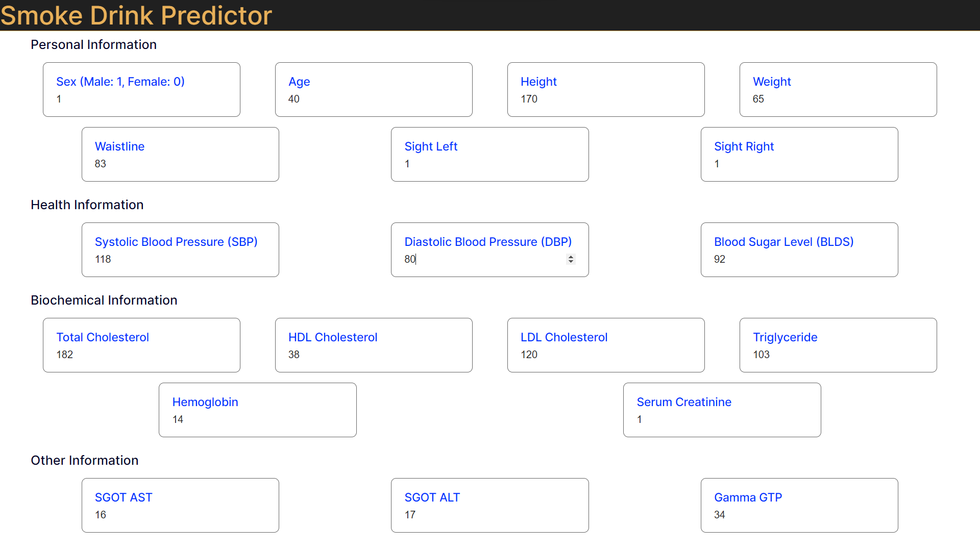
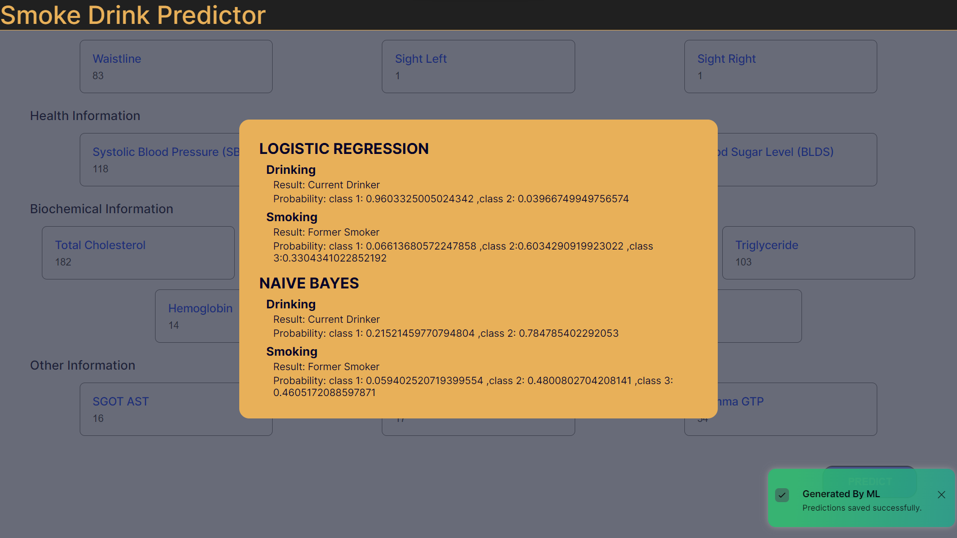
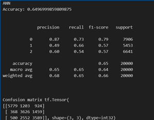
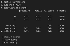
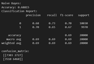
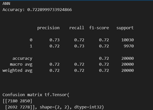
Often when patients are diagnosed with a respiratory problem or health condition, they are reluctant to reveal information regarding their smoking and drinking status, that is, whether they smoke or drink and if so, how frequently. There may be several reasons ranging from fear of dismissal or appearing as someone who is careless about personal health. In any case, this leads to misinformation and difficulty for medical practitioners in providing proper treatment. Therefore, there is a need for accurate knowledge of a patient’s smoking and drinking status without having to rely on the patient’s words for the same. It has been shown that this very information can be predicted based on several measurable body signals such as Blood Pressure, Cholesterol, Urine Proteins, and a few enzymes. Practitioners can use Machine Learning Models trained on this data available for several patients to predict the status of future patients. This report summarizes an attempt at the problem discussed above. Details will follow.
The dataset for the project is the Smoking and Drinking Dataset with body signal and has been sourced from Kaggle. This dataset was collected from the National Health Insurance Service in Korea and all personal information and sensitive data were excluded. The data contains 9,91,346 rows and 24 columns.
- Sex male, female
- Age round up to 5 years
- Height round up to 5 cm[cm]
- Weight [kg]
- Sight_left eyesight(left)
- Sight_right eyesight(right)
- Hear_left hearing left, 1(normal), 2(abnormal)
- Hear_right hearing right, 1(normal), 2(abnormal)
- SBP Systolic blood pressure[mmHg]
- DBP Diastolic blood pressure[mmHg]
- BLDS BLDS or FSG(fasting blood glucose)[mg/dL]
- Tot_chole total cholesterol[mg/dL]
- HDL_chole HDL cholesterol[mg/dL]
- LDL_chole LDL cholesterol[mg/dL]
- Triglyceride triglyceride[mg/dL]
- Hemoglobin hemoglobin[g/dL]
- Urine_protein protein in urine, 1(-), 2(+/-), 3(+1), 4(+2), 5(+3),(+4)
- Serum_creatinine serum(blood) creatinine[mg/dL]
- SGOT_AST SGOT(Glutamate-oxaloacetate transaminase) AST(Aspartate transaminase)[IU/L]
- SGOT_ALT ALT(Alanine transaminase)[IU/L]
- Gamma_GTP y-glutamyl transpeptidase[IU/L]
- SMS_stat_type_cd Smoking state, 1(never), 2(used to smoke but quit), 3(still smoke)
- DRK_YN Drinker or Not
It was observed that out of the 9,91,346 patients, around 6,00,0000 were non – smokers, which means that the proportion of patients who smoke or used to smoke is relatively small. To remove the oversampling, the number of non–smokers was reduced to 2,50,000 by random selection.
Plotting values in each column as a parameter vs. the smoking status of a patient, it was observed in the case of columns urine_protein, hear_left, and hear_right that the observed values lie in the normal range for smokers and non–smokers alike. Hence, these three parameters were not taken into consideration in making predictions. Removing Outliers Outliers are observations that differ considerably from other observations. Such data were removed from the dataset by deleting entries whose parameters had data points lying in the top 0.1% of the complete data. 8,433 such points were found and their removal brought down the number of entries to 6,30,472.
The mean, standard deviation and median of the data points for each parameter have been plotted in the figure below. The horizontal axis distinguishes smokers as ‘Never Smoked,’ ‘Former Smoker’ and ‘Current Smoker.’ We can see that all three values are more – or – less similar for all types of smokers.
- Blue: Mean
- Orange: Standard Deviation
- Green: Median
Outliers are observations that differ considerably from other observations. Such data were removed from the dataset by deleting entries whose parameters had data points lying in the top 0.1% of the complete data. 8,433 such points were found and their removal brought down the number of entries to 6,30,472.
Count plots were made for all the remaining parameters for a random sample of 1,00,000 patients to understand their distribution better. The plots for all three types of smokers emerged similar for most of the parameters, but there were slight exceptions like in the case of hemoglobin.
Along with relations to the smoking status, relations between the parameters themselves also provide important insights. A heatmap is a two-dimensional graphical representation of data where the individual values that are contained in a matrix are represented as colors. A heatmap was made to study relations among the parameters.
From the heatmap, we can see strong correlations between SBP – DBP, LDL_chole – tot_chole and SGOT_ALT – SGOT_AST. There was also a considerable correlation between sight_left – sight_right, which, being categorical variables (a variable that can take on only one of a small fixed list of values) were not plotted on the heatmap. So, we may consider reducing these parameters from 8 to 4 using methods such as PCA, SVD and LDA to reduce the number of dimensions. At the same time, we must be careful not to reduce the number of parameters too much because there already are only 22 parameters remaining to describe around 1,00,000 data – points. Keeping this in mind, parameters were reduced only in situations where one of the three methods (PCA, SVD, LDA) resulted in a data loss of less than 0.5%.
Data loss in each case was calculated using the formula: ▭("data_loss = 1–explained_variance" ["0" ] ) Finally, LDL_chole – tot_chole, SGOT_ALT – SGOT_AST and sight_left – sight_right were reduced to a single parameter each using LDA.
After the initial analysis and reduction of parameters, we proceeded to the Machine Learning Models.
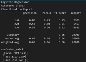
Logistic Regression is justified for predicting "isDrinker" in the dataset due to its compatibility with binary outcomes. There are 3 types of patients in the target class for smokers (non – smokers : 1, stopped smoking: 2, smoker : 3). However, Logistic Regression is generally used for binary classification. But, in the scikit learn library, the model has been extended to include multi – class classification. The model has been used in its default mode (‘auto’ for multi – class). Here is an exerpt from the documentation: “‘auto’ selects ‘ovr’ if the data is binary, or if solver=’liblinear’, and otherwise selects ‘multinomial’.”
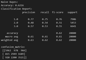
Naive Bayes methods are a set of supervised learning algorithms based on applying Bayes’ theorem with the “naive” assumption of conditional independence between every pair of features given the value of the class variable. More can be found here. Its capacity to handle both continuous and categorical data makes it suitable for variables like age, health metrics, and lifestyle indicators. Despite the assumption of feature independence, Gaussian NB performs well, particularly with limited dependencies. Its efficiency with smaller datasets, simplicity, and interpretability make it a practical choice.
The choice of a deep neural network with multiple hidden layers and specific activation functions (ReLU for intermediate layers and Sigmoid for the output layer) was taken for the following reasons:
- Complex Relationships: The dataset includes various health and lifestyle features, suggesting potential complex relationships. The deep architecture allows the model to learn hierarchical and intricate patterns, capturing nuanced dependencies among predictors.
- Non – linearity: ReLU (Rectified Linear Unit) is commonly used for hidden layers, introducing non-linearity essential for learning complex mappings. It enables the model to represent more intricate relationships between input features.
- Layer Size Variation: Gradually increasing the number of units in hidden layers (e.g., from 16 to 256) allows the model to capture increasingly complex representations of the data, promoting feature learning at different abstraction levels.
- Sigmoid Activation for Binary Classification: Using Sigmoid activation in the output layer is appropriate for binary classification tasks like predicting "is_Smoking" and "isDrinker." It squashes the output to a range between 0 and 1, representing probabilities.
- Categorical Crossentropy Loss: Categorical Crossentropy loss is appropriate when dealing with categorical classification tasks. It penalizes the model based on the difference between predicted and true class probabilities.
- Training and Evaluation: The model is trained for 30 epochs with a batch size of 128, and performance is evaluated on a separate test set. This ensures a balance between model training and evaluation, helping to identify potential overfitting.
