shuiyao / PyGIZMO

A light-weight, interactive Python/C library for wrangling, analyzing and visualizing cosmological simulation data.

PyGIZMO: Python APIs for the GIZMO Simulation

Introduction

PyGIZMO is a light-weight software that provides convenient APIs to cosmological hydrodynamical simulation outputs from the GIZMO code.

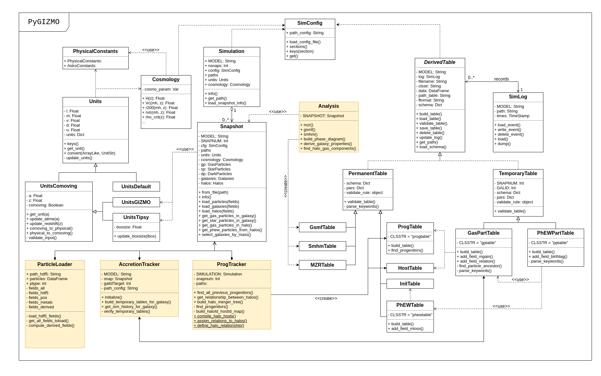
The main components of PyGIZMO include a data warehouse implementation, several high-level modules for scientic analysis and modules for data visualization.

PyGIZMO implements data pipelines that extract and transform simulation data from various sources with multiple formats into a coherent data warehouse that can be managed with a clean set of APIs. The simulation data includes the raw particle data from the simulation snapshots, galaxy catalogs generated from group finders, and record files that stores the run-time information of wind particles.

In addition, PyGIZMO implements several high-level functionalities such as generating halo merger trees and tracking galactic accretion that involves some intensive computations and heavily relies on efficient data pipelining. In particular, PyGIZMO provides unique supports to analyzing the outputs from the PhEW (Physically Evolved Winds) model, which is a novel sub-grid model in the GIZMO simulations that analytically propagates wind particles in the galactic halo.

Finally, PyGIZMO provides many plotting modules that enable quick inspection of the simulation data as well as making complicated figures for journal publications.

Future Works: Implement a set of APIs that interact with simulation data and specexbin, a C program for generating mock quasar absorption line spectra. Add modules that analyze the output spectra, e.g., fit line profiles to different ions in the spectra and obtain their physical properties such as column density, equivalent width, etc.

Quick Start

Requirements

PyGIZMO is built and tested with the following libraries:

#+CAPTION[Lists]: Pre-requisites

• Python 3.x
• numpy >= 1.19.0
• scipy >= 1.6.0
• pandas >= 1.2.0
• h5py >= 2.10.0
• matplotlib >= 3.3.0
• seaborn >= 0.11.0
• pyspark >= 3.1.1
• tqdm (optional, progress bar animation)

Installation

git clone http://github.com/shuiyao/PyGIZMO
cd PyGIZMO
pip install .

Examples

This jupyter notebook demonstrates several basic and advanced user cases of the program.

Load snapshots

>>> from pygizmo.snapshot import Snapshot
>>> model = "l25n144-test"
>>> snap = Snapshot(model, 98)
Snapshot: l25n144-test, snapnum: 98
>>> snap.redshift
0.2500000073365194
>>> snap.cosmology
{'Omega0': 0.3, 'OmegaLambda': 0.7, 'HubbleParam': 0.7}
>>> snap.get_units('tipsy', cgs=False).get('length')
35714.285714285725    
>>> snap.ngals
1469
>>> snap.ngas
2561261
>>> snap.select_galaxies_by_mass_percentiles(0.98, 0.985)    
       Npart   logMstar    logMgal
galId                             
48       728  10.860389  10.981041
95       722  10.888107  11.002301
589      673  10.881828  10.962551
827      690  10.871061  10.991914
841      727  10.918854  11.011083
889      676  10.914965  10.981414
936      653  10.907985  10.954995
>>> snap.load_gas_particles(['PId','Mass','galId','Tmax'])
>>> snap.gp.columns
Index(['PId', 'Mass', 'galId', 'Tmax'], dtype='object')
>>> snap.load_gas_particles(['PId','logT'])
Index(['PId', 'U', 'Ne', 'Y', 'logT'], dtype='object')

>>> from plotlib.map2d import DensityMap
>>> fig, ax = plt.subplots(1, 1, figsize=(8,8))
>>> map2d = DensityMap(snap, ax, zrange=(0.0, 1.0))
>>> map2d.add_layer_density_map(layer='temperature', ncells=(256, 256))
>>> map2d.add_layer_particles(verbose=True, skip=None)
>>> map2d.draw()
'''

Draw phase diagram

>>> from pygizmo import snapshot
>>> from plotlib.map2d import PhaseDiagram
>>> model = 'l25n144-test'
>>> path_grid = "/path/to/l25n144-test/tabmet_108.csv"
>>> fig, ax = plt.subplots(1, 1, figsize=(6,6))
>>> snap = snapshot.Snapshot(model, 108)
>>> rhot = PhaseDiagram(snap, ax)
>>> rhot.load_grid_data(path_grid)
>>> rhot.draw(annotate=True)        
>>> plt.show()

Make a movie of a single evolving halo

Configuration

The configuration file pygizmo.cfg (sample) controls many global parameters that defines and controls:

• The general behaviors of PyGIZMO
• The input formats and units of the simulation outputs
• Default settings of the plotting modules, i.e., plotlib

The configuration files consists of different categories, each with a set of parameters.

#+CAPTION[Lists]: Categories in the configuration file

Paths

The paths that are used in I/O

• pygizmo: Location of the PyGIZMO module.
• data: Location for the simulation raw outputs and some massive derived tables (e.g., phewtable, inittable).
• workdir: Location for derived and compiled results (e.g., grid data for the phase diagram, galaxy statistics), some permanent tables that are frequently loaded (e.g., progtable).
• tmpdir: Location for ‘cached’ data, e.g., temporary tables, halo particle data used for plotting.
• figure: Output location for figures.

Schema

The schema for different source data.

Verbose

The numeric values for different levels of verbosity.

Units

The default units for length, mass, velocity and magnetic field strength. The GIZMO/GADGET tradition uses 1 kpc, 10^10 M_solar, 1 km/s and 1 Gauss.

Cosmology

Cosmological parameters. Should be the same as in the simulation.

Default

A list of default values

• logT_threshold: The log temperature that separates cold and hot gas.

Simulation

Some attributes specific to each simulation

• snapnum_reference: Defines the ascales of all simulation snapshots.
• n_metals: Total number of elements in the Metallicity field.
• elements: Ordered list that defines the name of elements in the Metallicity field.

Ions

TODO. Properties of several important ion spectral lines.

Zsolar

Abundances of various elements in the solar atmosphere. Often used to normalize metallicity.

HDF5Field

Shortnames for HDF5 fields

HDF5ParticleTypes

The numerical value that corresponds to a specific particle type. Particles of any specific type are stored under PartType#/ in the HDF5 file. By default, 0, 1, 4, 5 correspond to gas particles, dark matter particles, star particles and black hole seed particles (if exist). In zoom-in simulations, 2, 3 usually correspond to dark matter particles at finer levels of resolutions.

Derived

A list of quantities that are not stored in the HDF5 files but can be derived from other HDF5 fields. For example, logT (log temperature) is a crucial gas property that needs to be derived from the U (internal energy), Ne (electron abundance) and Y (helium abundance) fields.

API Example:

>>> from config import SimConfig
>>> cfg = SimConfig('/path/to/the/config/file.cfg')
>>> cfg.sections()
['DEFAULT', 'Paths', 'Schema', 'Verbose', 'Units', 'Cosmology', 'Default', 'Simulation', 'Ions', 'Zsolar', 'HDF5Fields', 'HDF5ParticleTypes', 'Derived']
>>> cfg.keys('Simulation')
['snapnum_reference', 'n_metals', 'elements']
>>> cfg.get('Simulation', 'elements')
'Z,Y,C,N,O,Ne,Mg,Si,S,Ca,Fe'

Plotlib: Convenient APIs for Fine Tuning Figures for Journal Articles

The current module implements the following classes:

MultiFrame: An easy interactive tool that manages figure layouts

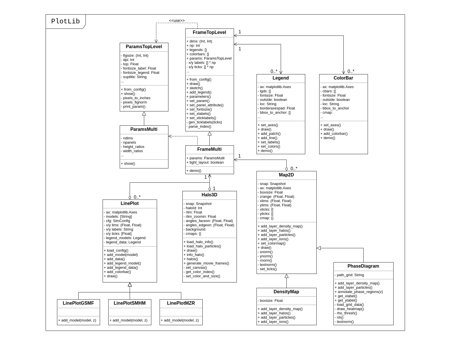
The MultiFrame class defines the general layout of a figure through a set of parameters and APIs. One could always call the sketch() method to checkout the current layout of the figure, and then fine tune the parameters iteratively before adding data to the figure.

Once the layouts are finalized, one can call the draw() method, which returns fig and axs.

PlotLib provides two additional classes can be used to easily customize figure legends and colorbars:

• Legend: Easily customizing multiple legends to MultiFrame
• ColorBar: (TODO) Easily customizing multiple colorbars to MultiFrame

Here is demo for several user cases:

I. 2 x 2, tight layout, identical panels

   +-------+-------+
   |       |       |
 y |       |       |
   |       |       |
   +-------+-------+
   |       |       |
 y |       |       |
   |       |       |
   +-------+-------+
       x       x

>>> frm = FrameMulti(2,2,tight_layout=True)
>>> frm.set_xlabels('x', which='row')
>>> frm.set_ylabels('y', which='col')

II. 2 x 2, independent panels

   +-------+    +-------+
   |       |    |       |
 y |       |  y |       |
   |       |    |       |
   +-------+    +-------+
       x            x
   +-------+    +-------+
   |       |    |       |
 y |       |  y |       |
   |       |    |       |
   +-------+    +-------+
       x            x

>>> frm = FrameMulti(2,2,tight_layout=False)
>>> frm.set_param('hspace', 0.25)
>>> frm.set_xlabels('x')
>>> frm.set_ylabels('y') # which = 'all' by default
>>> frm.sketch()

III. Main and side panels

    +-------+---+
    |       |   |
 y1 |       |   |
    |       |   |
    +-------+---+
 y2 |       | x
    +-------+
        x

>>> frm = FrameMulti(2,2)
>>> frm._params.height_ratios = [4, 1]
>>> frm._params.width_ratios = [4, 1]
>>> frm.set_xlabels('x', which=[(1,0),(0,1)])
>>> frm.set_ylabels('y1', which=(0,0))
>>> frm.set_ylabels('y2', which=(1,0))
>>> frm.axisON[3] = False
>>> frm.sketch()

IV. (2) x 3 panels

    +-------+-------+-------+
    |       |       |       |
 y1 |       |       |       |
    |       |       |       |
    |       |       |       |
    +-------+-------+-------+
 y2 |       |       |       |
    +-------+-------+-------+
       x        x       x

>>> frm = FrameMulti(2,3,tight_layout=True)
>>> frm._params.height_ratios = [4, 1]
>>> frm.set_xlabels('x', which='bottom')
>>> frm.set_ylabels('y1', which=(0,0))
>>> frm.set_ylabels('y2', which=(1,0))
>>> frm.sketch()

V. 2 x 2, tight layout with legends

   +-------+-------+ 111
   |       |       | 111
 y |       |       |
   |       |       |
   +-------+-------+
   |    333|       |
 y |       |       |
   |       |       | 2222
   +-------+-------+ 2222
       x       x

>>> frm = FrameMulti(2,2, True)
>>> frm.set_xlabels('xlabel')
>>> frm.set_ylabels('ylabel')

>>> lgd1 = Legend()
>>> lgd1.add_line("lgd1:black line")
>>> frm.add_legend(lgd1, which="upper right", loc="upper right")

>>> lgd2 = Legend()
>>> lgd2.add_patch("lgd2:red patch", fc='red')
>>> frm.add_legend(lgd2, which="lower right", loc="lower right")

>>> lgd3 = Legend()
>>> lgd3.add_line("lgd3:thick blue dashed line", "blue", "--", 2)
>>> frm.add_legend(lgd3, which="lower left", loc="upper right")

>>> frm.set_param('right', 0.80)
>>> frm.sketch()

LinePlot: Interface for line-type plot.

LinePlot provides a unified interface for making line-type plot that includes data from various sources (both models/simulations and observational/experimental data) in a single panel. A popular user case is to compare the GSMFs from many simulations to observational data in a same plot.

It relies on two external files as input:

• A configuration file (e.g., ”lineplot.cfg”) that defines the default panel-level attributes (e.g., the x/y limits, labels, tick formats, fontsizes) of different types of plots.
• A tabular file that defines the color/style schema for various models. The same schema could be used for various types of plots for consistency. Here is an example table:

model	color	style	size	label
l25n288-mfm	red	-	2	MFM-Hres
l25n144-mfm	red	–	1	MFM-Lres
l25n288-sph	blue	-	2	SPH-Hres
l25n144-sph	blue	–	1	SPH-Lres
baldry12	black	o	12	Baldry+12

Here are some of the advantages of using LinePlot

• Maintain a consistent color/linestyle schema for each model through a report/paper.
• Easily build and reload template layouts for various types of plots.

Currently several types (most common ones in extragalactic astronomy) of plots have implemented this interface:

• LinePlotGSMF: Galactic stellar mass functions
• LinePlotSMHM: Stellar mass - halo mass functions
• LinePlotMZR: Mass-metallicity relations

Map2D: Customizing multi-layer 2D maps for simulations

Map2D is an interface for two-dimensional maps (z = f(x, y)). Most common instance is a density map (2D histogram).

Currently two classes of figures have implemented Map2D:

DensityMap: Draw density field for a snapshot

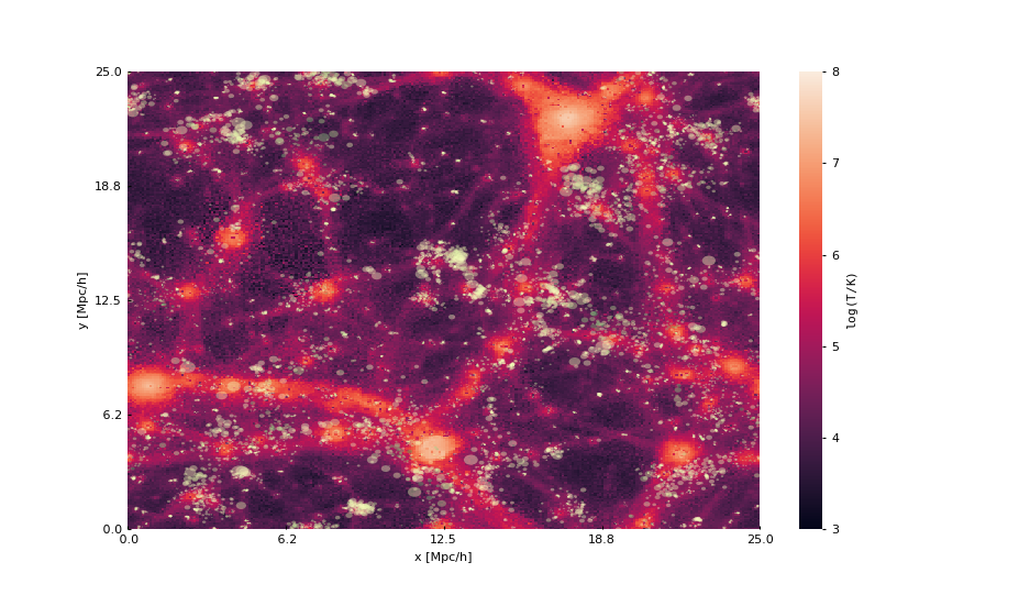
The base layer shows the mass density or temperature distribution of snapshot. The region to display can be a slice from the simulation and at a user defined resolution level.

A few additional layers can be added to the base layer.

Galactic halos

By default, galactic halos within a given mass range can be displayed as circles whose sizes correspond to the physical radius of the halos.

Particles

A layer of selected particles. Often we overplot wind particles on top of the density map to show the prevalence of galactic winds in a snapshot.

(TODO) Contour of different ions (e.g., HI, OVI)

Note that different ions are sensitive to different physical conditions such as density, temperature and metallicity and therefore trace different structures.

PhaseDiagram: Customizing multi-layer phase diagrams

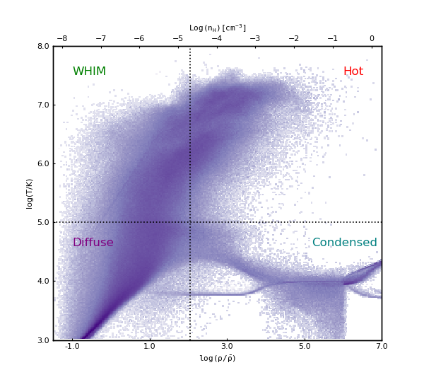
The mass distribution of gas particles in the density-temperature space.

Like in a DensityMap, PhaseDiagram allows a particle layer and a ion contour layer.

Halo3D: Generating 3D particle layouts for galactic halos

Draw an overall view of the configuration of various types of particles in a selected halo, and two additional views that zoom in on the center of the halo.

One can make a movie (e.g., Evolution of a galaxy) showing the evolution of the halo over time by identifying and showing its progenitors in previous snapshots.

Class diagram

Galaxy and Halo Properties

The Analysis classes provides functions that compute key diagnostic statistics and analytics for galaxy and halo properties, such as the galactic stellar mass functions (Gsmf), stellar mass - halo mass functions (Smhm), mass metallicity relation (Mzr), halo gas components (HaloGasComponents) and halo radial profiles (RadialProfile). The results are often saved as permanent tables in designated locations that can be used by the plotting modules for making scientific figures.

Example: Galactic stellar mass function at multiple redshifts

The following script generates the galactic stellar mass functions at four redshifts from a simulation, saves the result to the work-dir and compares the results with observational data.

Galactic stellar mass function at z = 0,1,2,4

from simulation import Simulation
from analysis import Gsmf
from plotlib import FrameMulti
from plotlib.lineplot import LinePlot, LinePlotGSMF

# Generate the GSMFs at four redshifts
gsmf = Gsmf("l25n144-test")
redshifts = [0.0, 1.0, 2.0, 4.0]
gsmfs.compute(z=redshifts, overwrite=True)

# Make plot
frm = FrameMulti(2, 2, tight_layout=True) # 2 x 2 share-xy
frm.set_xlabels('$\log(M_{gal}/M_\odot)$', loc='bottom')
frm.set_ylabels('$\Phi(M)dMdz$', loc='left')
frm.set_xticks([10.0, 10.5, 11.0, 11.5, 12.0])
frm.set_yticks([-4., -3., -2., -1., 0.0])
frm.draw()

for i, z in enumerate(redshifts):
  lines = LinePlotGSMF(ax=axs[i], models="models.dat")
  lines.add_model('l25n144-test', z=z)
  lines.draw()

To compare the results with other simulations and observational data, replace the last section with (with a input file like this one):

models = ['l25n144-test', 'l25n288-test', 'l25n144-final', 'l25n288-final']
observations = ['baldry12', 'tomczak14', 'tomczak14', 'song16']

for i, z in enumerate(redshifts):
  lines = LinePlotGSMF(ax=axs[i], models="models.dat")
  for model in models:
    lines.add_model(model, z=z)
  lines.add_data(observations[i])
  lines.draw()

Design notes: derived tables and log files

Since some of the computations for derived properties of galaxy and halo properties can be expensive, PyGIZMO automatically saves the results into tabular files at designated locations and keep tracks of any expensive operation that has already been performed on a simulation basis. These results can then be loaded into other modules without having to be re-computed.

PyGIZMO implements this idea using two classes, DerivedTable and SimLog, for each simulation/model. Whenever a DerivedTable has been computed and saved, an entry is written into the SimLog with detailed information on how the table was generated (e.g., the parameters that was passed to the DerivedTable.build_table() method). At any time when a particular result is needed, DerivedTable.load_table() will check the SimLog to see if the table has already been created with the same parameters. If so, unless the keyword overwrite is set to True, the existing result will be loaded.

The DerivedTable has two sub-classes, PermanentTable and TemporaryTable. The permanent tables are often results that are deterministic and often used, such as the galactic stellar mass functions, merger trees, and the many simulation-level inputs to the accretion tracking engine. The temporary tables often have limited usage, are intermediate outputs of a long data pipeline, or depend on user defined parameters.

Merger Trees

<sec:mergertree>

Halo Merger Trees

Halo merger trees define the relation between two halos at different time. In a simulation, a halo is uniquely determined by a pair Halo(haloId, snapnum), where haloId is the ID of the halo at a particular snapshot (snapnum).

A halo merger tree reconstructs the assembly history of any halo from a snapshot, locating its main progenitor in all previous snapshots since its formation and defines the relations between all halos at a snapshot to the progenitor at the same snapshot.

The merger trees and the related properties are managed with the ProgTracker class in progen.py.

Algorithm

First of all, in each snapshot, one finds the host halo for any halo in the snapshot. The center of a halo must reside within the virial radius of its host halo, which is more massive. The result is saved in a PermanentTable named hostmap.

The main progenitor of any halo in an earlier time is defined as the halo that contains most of its dark matter particles at that snapshot. Since the halo finder only identifies strucutres over a certain mass as halos, the progenitor is not guaranteed to be found if it has not assembled enough mass to be classified as a halo.

A halo from an earlier time is said to be captured by another halo, if most of its mass ends up in a satellite halo of the main descendent of that halo.

Example

Galaxy Merger Trees

Implementation

Output Create stars_snapnum.csv for each snapshot

column	source	description
snapnum	-	Integer
starId	HDF5	PID for each star particle
mass	HDF5	Mass at this snapshot
galId	grp	galId at this snapshot
haloId	sogrp	haloId at this snapshot
mainId	Derived	The Unique galId for the simulation
initId	Derived	First galId after the star formed

The mainId file:

column	dtype	description
mainId	int64
snapnum	int32
galId	int32
hostId	int32
Mstar	float32	Stellar Mass
Mtot	float32	Galaxy Mass
Mhost	float32	Host Halo Mass
mainIdNext	int64	The mainId of its descendent

Find the parent and snaplast of a mainId First of all, maybe this information is redundant.

Create a temporary table: galId -> galIdNext

MainId -> galId -> galIdNext (Join, groupby and sortby sum(mass)) -> MainIdNext (Unique)

Last snapshot: stars having mainId This snapshot: These stars having different mainId

Brute Force:

• Left join by starId to last snapshot, compare mainIdlast and mainId
• Group by mainIdlast, pick the mainId as max(mass)
  • Expect in most cases mainIdlast == mainId
• Or. Group by galIdlast, find the galId in the next snapshot
  • galId uniquely determines mainId in the next snapshot

Example: snap i, mainId j: [[initId1], [InitId2], [InitIdj]]

Relation between two galaxies at different time Task: Find the direct descendent of g0 at a later time t1.

Galaxy g0: (snapnum=t0, galId=0) Galaxy g1: (snapnum=t1>t0, galId=1)

At time t0, all stars in g0 has the same galId and mainId. At time t1, they have different galId(t0) and mainId(t0), but supposedly most of them end up in a single galaxy g0’. If g0.mainId == g0’.mainId, R(g0, g0’) = ‘SELF’. If g0.mainId <> g0’.mainId, R(g0, g0’) = ‘MERGE’.

Define R(g0, g1) according to the relation between g0 and g0” g0” at t0 is backtracked from g0’:

• g0”.mainId = g0’.mainId is found.
  • R(g0, g1) = ‘SELF’ if g0”.mainId == g0.mainId
  • R(g0, g1) = ‘SAT’ if g0”.galId == g0.hostId
  • R(g0, g1) = ‘CEN’ if g0”.hostId == g0.galId
  • R(g0, g1) = ‘SIB’ if g0”.hostId == g0.hostId not in [g0”.galId, g0.galId]
  • Else: R(g0, g1) = ‘NGB’
• Not found. R(g0, g1) = ‘SELF’ Reason: Most g0 ends up in g0’. g0 formed even before the mainId of g0’. So even if g0’.mainId formed apart from g0, winds from g0 get back to g0’s dscendent.

Global variables maxMainId: Int. Counter for the global maximum mainId spAll: DataFrame. All star particles.

Procedure

1. Generate stars_$snapnum.csv Table

generate_star_history(model, start=0): Driver program. Start from earlier snapshot (start) and move forward in time. If start is not 0, read data from the last snapshot that has been processed.

• process_snapshot(model, i): Update with the i-th snapshot.
  • load_snapshot(snapname, grpname): Load HDF5 and grp data
    • load_galaxies(fname, numPart): Load grp data.
  • find_mainId_for_gals(spAll): Assign for each galaxy some mainId, if it is the mainId of most stars (by mass) in the galaxy.
  • update_mainId_of_stars(spAll, mainIds): Update mainId for each star as the mainId of its host galaxy at this snapshot.

1. Generate galmainid Table

Pandas is likely sufficient for this task. galtree.py:build_mainId_table()

1. Find the relations between two halos at different times

Method I. Find the most massive progenitor of any halo gal1 at z1 at z0 (z0 > z1), gal1’. Define the relation between gal1 and any halo at z0 by the relations between gal1’ and those halos (SELF, SIB, SAT, CEN, NGB). This method does not require the mainId information. (galId, snapnum<snapnum0) -> (galId, hostId) In total, ngals * (snapnum0-1) lines. I can use dark matter to trace halos.

Caveats

• Tidally stripped stars make up around 50% of the total stellar mass. Therefore, we need to make sure that:
  • Assign new mainId to a star only if it is in a SKID galaxy
  • Map mainId at any time only to SKID galaxy (galId != 0)

Accretion Tracking Engine

<sec:accretionTracker>

Analyzing the history of gas accretion into a galaxy is critical to understanding galaxy formation and evolution. The accretion tracking engine in PyGIZMO reconstructs the history of selected gas particles from a wide range of simulation outputs and classifies their accretion events into several categories that are physically motivated. The engine tracks selected gas particles across previous snapshots and analyzes their interactions with the galactic halos and wind particles over time.

Basic Usage

The accretion.AccretionTracker class provides most of the public APIs for tracking accretion.

This following example creates a pandas DataFrame that tracks the accretion histories for all gas particles in the interstellar medium of a galaxy at z = 0.

from snapshot import Snapshot
from accretion import AccretionTracker

# Create an instance of the AccretionTracker from a snapshot (z=0)
model = "l25n144-test"    
snap = snapshot.Snapshot(model, 108)
act = AccretionTracker.from_snapshot(snap)

# Prepare all required permanent tables. Load if already existed, otherwise build new.
act.initialize()

# Build temporary tables for selected particles from a galaxy specified by galIdTarget. Will take a while if the tables have not yet generated.
act.build_temporary_tables_for_galaxy(galIdTarget)

# Run the engine and generate result
mwtable = act.compute_wind_mass_partition_by_birthtag()

The resulted table can be used to answer many questions. For example, to find the total amount of wind recycling divided into the different categories:

mwtable.groupby('birthTag')['Mgain'].sum()

Algorithm

Classification scheme

<sec:categories>

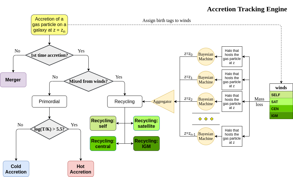
This following diagram demonstrates the algorithm for classifying gas particles according to their accretion history. In a typical scenario, one looks at all the gas particles (form a list of particle IDs, i.e., pidlist) that recently accreted into a galaxy (target galaxy) at some time, and classifies them into several accretion mode according their evolution histories at earlier times before accretion. PyGIZMO tracks each of the particle by their unique particle ID over previous snapshots and extracts key information that help classify the particle into one of the following accretion modes:

• Merger: The particle was found in another galaxy at some previous time (already accreted at least once prior to the current accretion event).
• Primordial: For first time accretion, the original component of a gas particle is classified as primordial accretion, which has two sub-categories
  • Cold accretion: If the maximum temperature that the gas particle ever reached was below 10^5.5 K (controlled by (logT_threshold)).
  • Hot accretion: If the maximum temperature was higher.
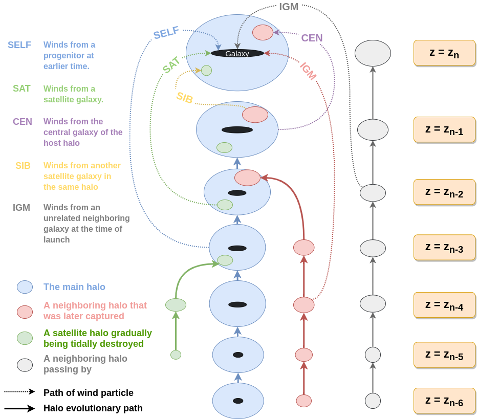
• Recycled: For first time accretion, the mixed-in wind materials are treated separately from primordial accretion. The wind materials are further classifed according to the relation between the progenitor of the target galaxy progenitor and the galaxy where the winds originated from birth site.
  • Recycled from self: The wind materials originated directly from the direct prognitor of the target galaxy at some earlier time.
  • Recycled from central: The birth site was the central galaxy of the progenitor.
  • Recycled from satellite: The birth site was the satellite galaxy of the progenitor
  • Recycled from IGM: The birth site and the progenitor were unrelated at the time of wind launch.

Tracking wind component

<sec:windTracking>

More about tracking recycled materials: In a PhEW simulation, a normal gas particle may constantly get wind materials from different neighboring wind particles. Tracking every single mass flow between normal gas particles and wind particles and keeping track of where the wind particles came from will take too much disc space and is therefore impractical. Instead, we provide an approximate solution (‘Bayesian machine’ in the diagram) relying on computing the posterior probability of a gas particle getting materials from each of the recycled categories between two snapshots. See this journal article for details.

Particle splitting

<sec:particleSplitting>

In later version of the PhEW, a gas particle splits into two halves when its mass grows to over 3 times its original mass. One of the newly spawned particle will inherit the particle ID while the other one will have a new unique ID. The simulation outputs each of the splitting event into a log files like “split.snapnum”. The problem is, how to reconstruct the split history of any given gas particle from these files?

<def:generation> Definition of /generation/: Tracing back in time and starting from 0, the generation of the particle increases by 1 every time when it splitted in the past. If the particle was spawned at some earlier time from a parent, the generation will keep increasing for the parent.

The following example tracks the generation of a particle with PId = 3, which was spawned from another particle with PId = 12, which was then spawned from PId = 15. The particle splitted at snapnum = 106 and snapnum = 103.

snapnum:     108 107 106 105 104 103 102 101 100 099 098
ParticleID:  3   3   3   3   3   3   12  12  12  12  15 
Split                X           X   X       X       X
generation:  0   0   1   1   1   2   3   3   4   5   6

The particle was at generation = 6 at snapnum = 98. Therefore we assume that only 1/32 (2^-gen) of the mass of particle PId = 15 ended up in particle PId = 3 at snapnum = 108.

Firstly, a permanent table, splittable, is built for each simulation (Simulation.build_splittable()). Each entry corresponds to a split event and keeps the newly spawned particle ID (PId), the ID of the particle that splitted (parentId), the next snapnum after the split (snapnext) and the generation of the splitting particle at this particular splitting event (parentGen).

Then, for a selection of particles, a temporary table, ancestors, which basically reconstructs the above diagram, is built with AccretionTracker._find_particle_ancestors(splittable, pidlist)

In each snapshot, AccretionTracker.build_gptable() loads all particles in the pidlist as well as their parents at that snapshot. The mass of each particle is reduced to match the generation number. For example, using the diagram above, at snapnum = 102, particle(3) did not exist yet, so the program looks for its parent particle(12) and reduce its mass to 1/8.

At any time, one particle could be the parent of multiple particles from later time. In these cases, information of the parent particle is copied multiple times for each of its descendents. However, the generation number for these descendents may not be the same. For example, the following diagram demonstrates the history of particle(4):

snapnum:     108 107 106 105 104 103 102 101 100 099 098
ParticleID:  4   4   4   4   4   4   4   4   12  12  15 
Split                                X       X       X
generation:  0   0   0   0   0   0   1   1   2   2   3

In the end, the final gptable should contain len(pidlist) unique PIds, each having one entry for each snapshot.

Implementation

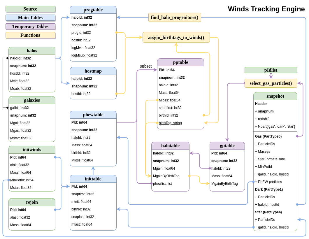
The accretion tracking engine relies on a set of permanent tables that need to be computed once for each simulation and a set of temporary tables that need to be constructed each time when one selects a new target halo from a snapshot. The following diagram demonstrates the workflow.

Data structures and schema

#+CAPTION[Table]: A list of Tables

Table	Format	Path	Sources	Description
inittable	CSV	$DATA	snapshot, initwinds, rejoin	Wind events (launch/rejoin)
phewtable	parquet	$DATA	snapshot, inittable, halos	PhEW particles
progtable	CSV	$WORK	snapshot, halos	Halo progenitors at earlier times
hostmap	CSV	$WORK	halos	The host for each halo
splittable	CSV	$WORK	split	Particle splitting event
gptable	parquet	$TMP	snapshot, halos	History of gas particles from the target
pptable	parquet	$TMP	snapshot, phewtable	History of relevant PhEW particles
halotable	CSV	$TMP	gptable, pptable, halos	Relevant Halos

Notes:

• The source column indicates the raw data from which the table is built.
• Default paths are defined in the configuration file.

Permanent tables The phewtable parquet table (Simulation.build_phewtable) #+CAPTION[Table]: phewtable

Field	dtype	Description
PId*	int64	Unique particle ID of a wind(PhEW) particle
snapnum	int32	Id of any snapshot in which PId is a wind
Mass	float64	Mass of the particle at snapnum
haloId	int32	haloId of the particle at snapnum
(Mloss)	float64	Mass loss since the previous snapshot
(birthId)	int32	The birthplace of the PhEW particle

It’s a gigantic table that needs to be frequently queried. It contains the attributes, such as mass and haloId, of all PhEW particles in any snapshot. The Mloss field is derived for each particle (PId) over time. Assume at each snapshot, a total mass of Mloss was lost from the PhEW particle (PId) to the halo (haloId) where it was found at that snapshot.

The inittable CSV table (Simulation.build_inittable()) #+CAPTION[Table]: inittable

Field	dtype	Description
PId*	int64	Unique particle ID of a wind(PhEW) particle
snapfirst	int32	The snapshot before becoming winds
minit	float64	Initial mass
birthId	int32	haloId of the halo in snapfirst
snaplast	int32	The last snapshot
mlast	float64	Mass when the particle appeared the last time

This table keeps records of all wind events in a simulation, such as when and where a wind particle was launched, the last time a wind particle appeared before fully evaporated, the mass of a wind particle at birth and death.

The progtable CSV table (Snapshot.build_progtable()) #+CAPTION[Table]: progtable

Field	dtype	Description
haloId*	int32	Unique haloId in the single snapshot
snapnum	int32	Id of any previous snapshot
progId	int32	haloId of the progenitor in snapnum
hostId	int32	haloId of the host halo of the progenitor
logMvir	float32	Virial mass of the progentor
logMsub	float32	Total mass of the host

This table defines the prognitor of any halo from a snapshot in the previous snapshot. Recursively quering the table finds all previous progenitors of any given halo. We use this table to define the relation between any halo at a given snapshot and any halo in a previous snapshot, using progen.get_relationship_between_halos()

The hostmap CSV table (Simulation.build_hostmap())

This maps (snapnum, haloId) to hostId, the host galaxy/halo of the haloId at snapnum.

The splittable CSV table (Simulation.build_splittable()) #+CAPTION[Table]: splittable

Field	dtype	Description
PId*	int64	Unique particle ID
parentId	int64	The ID of its parent from whom it was split
Mass	float64	The mass of the parent before splitting
atime	float32	Time of splitting
snapnext	int32	Next snapshot since splitting
gen	int32	The generation at the current time

Temporary tables The temporary gptable Parquet table (AccretionTracker.build_gptable())

#+CAPTION[Table]: gptable

Field	dtype	Description
PId*	int64	Unique particle ID of a gas particle
snapnum	int32	Id of any previous snapshot
Mass	float64	Mass of the gas particle at snapnum
haloId	int32	haloId of the particle at snapnum
(Mgain)	float64	Total mass gained since the previous snapshot

It tracks the locations and properties of all selected gas particles (e.g., from a single galaxy at some time) in all the previous snapshots since the beginning of the simulation.

If the gas particle did not exist at any snapshot, find its parent at that snapshot (defined in the splittable).

If the particle has splitted before, reduce the Mass be a factor of 2^-gen, where ‘gen’ is the generation number of the particle.

Finally, a ‘Mgain’ field is computed as the total mass that the particle gained since the last snapshot, using a window function on each PId. AccretionTracker.compute_mgain_partition_by_Pid(gptable)

The newly generated table is saved as gptable_{:03d}_{:05d}.parquet, where ‘:03d’, ‘:05d’ are snapnum and galIdTarget, respectively.

1. The temporary pptable Parquet table (AccretionTracker.build_pptable(inittable, phewtable))

#+CAPTION[Table]: pptable

Field	dtype	Description
PId*	int64	Unique particle ID of a wind(PhEW) particle
snapnum	int32	Id of a snapshot
haloId	int32	haloId of the particle at snapnum
Mass	float64	Mass of the particle at snapnum
(Mloss)	float64	Mass loss since the previous snapshot
snapfirst	int32	The first snapshot
birthId	int32	haloId of where it is born
(birthTag)	str	Relationship tag of its birth halo

A subset of the gigantic phewtable with a selection of PhEW particles. A PhEW particle is selected if it ever appeared in any of the halos in the gptable. The table should contain a complete record for each selected PhEW particle, i.e., any snapshot in which the particle existed.

The ‘Mloss’ field is computed as the total mass that the particle lost since the last snapshot, using a window function on each PId.

For each PhEW particle, a birthId indicating its birth galaxy, is found from the inittable.

Finally, a birthTag is generated that defines the relationship between the birth galaxy and the target galaxy. This is done with: AccretionTracker.define_halo_relationship(progId,progHost,haloId,hostId)

The newly generated table is saved as pptable_{:03d}_{:05d}.parquet, where ‘:03d’, ‘:05d’ are snapnum and galIdTarget, respectively.

Procedure

Selecting particles

Select the particles that we want to track. The list of their particle IDs (pidlist) is an input to the AccretionTracker. Depending on the user case, the particles could be:

• Recently accreted particles on a galaxy. API: pidlist = Snapshot.get_recent_accretion(galIdTarget) (TODO)
• Current ISM particles within a galaxy(galIdTarget) API: pidlist = Snapshot.get_gas_particles_in_galaxy(galIdTarget)

Note that, if the particles do not come from a same galaxy, one needs to get a list of all of their host galaxies and build the temporary tables for every single galaxy individually.

Build/Load permanent tables

AccretionTracker.initialize()

Build temporary tables for any galaxy(galIdTarget)

AccretionTracker.build_temporary_tables_for_galaxy(galIdTarget)

1. Build the splitting histories of each particle in the pidlist.
   • AccretionTracker._find_particle_ancestors(splittable, pidlist)
   • This creates a temporary table AccretionTracker._ancestors
2. Build the gptable.
   • AccretionTracker.build_gptable(pidlist)
   • Load gas particles (or their parents) from each snapshot
   • Compute the total mass they gained between two snapshots
3. Build the pptable.
   • AccretionTracker.build_pptable(inittable, phewtable)
   • Select all PhEW particles that potentially interacted with the particles in the pidlist, from the phewtable.
   • Find the birth galaxy for each PhEW particle using information from the inittable.
   • Compute the mass loss of each PhEW particle between any two consecutive snapshots.
   • Add a birthTag to each PhEW particle that defines the relation between its birth galaxy and the target galaxy(galIdTarget). This operation needs gptable, progtable and hostmap.

Classify and accumulate wind materials over time

AccretionTracker.compuate_wind_mass_partition_by_birthTag()

The algorithm is here. For the purpose of description here, assume all wind materials lost from the PhEW particles are deposited uniformly in the halo (the prior is unity).

For each snapshot:

1. Compute the total amount of wind materials deposited into each halo by PhEW particles since the last snapshot.
2. Divide the amount into categories according to the birthTag of the PhEW particle.
3. Find for each halo, the gas particles that it hosted at that snapshot.
4. Compute the wind materials that those gas particles gained since the last snapshot, by category.
5. Accumulate over time for each gas particle.

Quasar Absorption Line Spectra

Future work.

Scalable Data Pipelines with Apache Spark

The performance bottle-neck for the accretion tracking engine is building the temporary tables.

https://github.com/tabaer/pbstools/blob/master/bin/pbs-spark-submit https://www.osc.edu/~troy/pbstools/man/pbs-spark-submit

References

The GIZMO Simulation Code

The Physically Evolved Winds (PhEW) Model, Journal Article, I. Model

The Physically Evolved Winds (PhEW) Model, Journal Article, II. Implementation