shivangg / picknplace

The pick and place challenge

Project: Kinematics Pick & Place

Working GIF

1. Kinematics Analysis

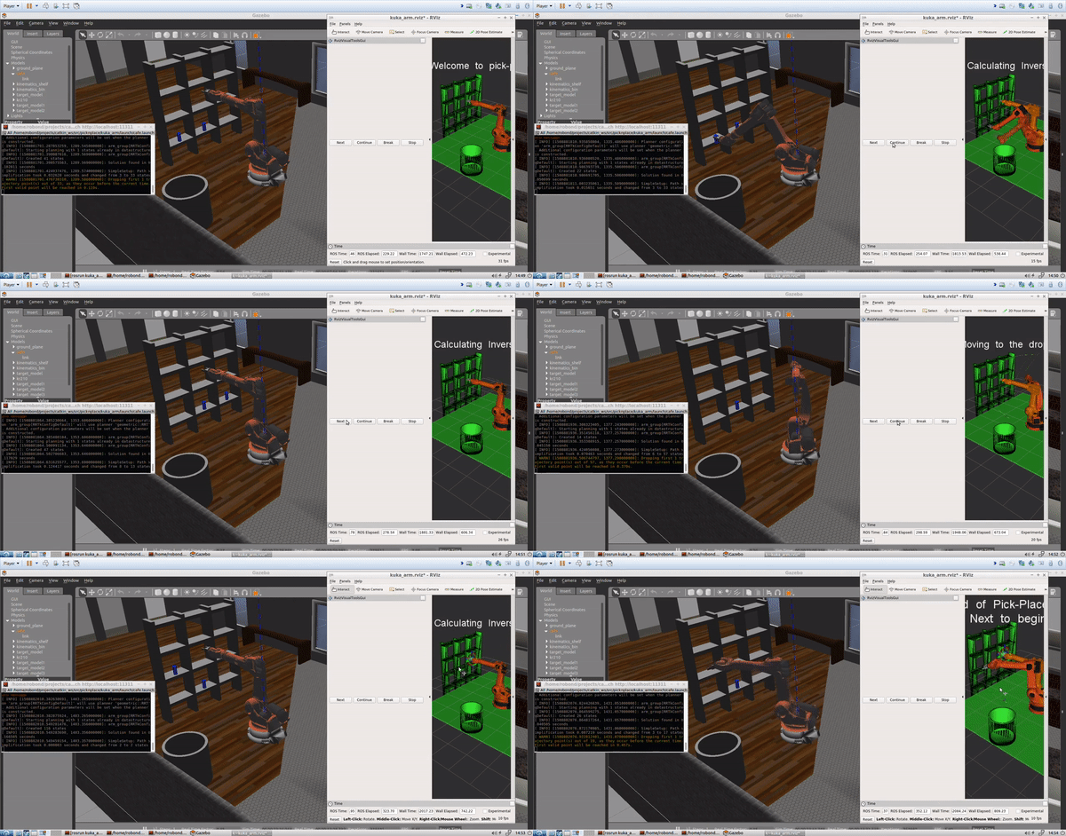
Here is the YouTube video showing the pick and plcace operation using the KR210 robotic arm

The diagrammatic representation of the joints in the KR210 at the initial state

Following steps need to be followed to successfully find the IK solution of the robotic arm.

1. Find a1, a2, a3, d4, dg

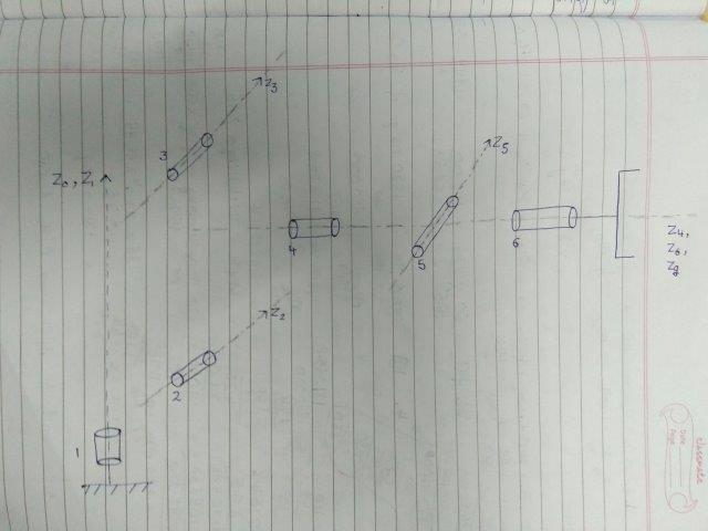
####Joints of KR210

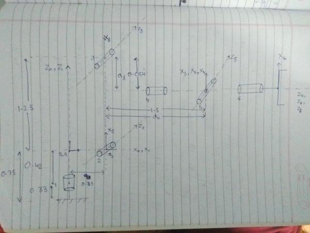
Find the 3D coordinates of the six joints and the gripper using the kr210.urdf.xacro file. The XYZ reading are relative to the parent link so we take the cumulative sum of the readings.

2. Make a python dictionary of known D-H parameters s.

The D-H Parameter Table

To calculate the DH parameters of the KUKA kR210 the URDF file kr210.xacro.urdf was used.

Link(i)	alpha( i-1 )	a( i-1 )	d( i-1 )	theta( i )
1	0	0	0.75	q1
2	-pi/2	0.35	0	q2 - pi/2
3	0	1.25	0	q3
4	-pi/2	-0.054	1.5	q4
5	pi/2	0	0	q5
6	-pi/2	0	0	q6
G	0	0	0.303	0

Storing these parameters as dictionary in python.

s = {
                alpha0: 0       , a0: 0     , d1: 0.75,    
                alpha1: -pi/2.   , a1: 0.35  , d2: 0. ,  q2: q2 - pi/2.,  
                alpha2: 0.       , a2: 1.25  , d3: 0. ,    
                alpha3: -pi/2.   , a3: -0.054, d4: 1.5,    
                alpha4: pi/2.    , a4: 0.     , d5: 0.,    
                alpha5: -pi/2.   , a5: 0.     , d6: 0.,    
                alpha6: 0.       , a6: 0.     , d7: 0.303 , q7: 0.   
        }

3. Compose the homogeneous transform matrices using the D-H parameters

To compose the matrix using the DH parameters for calculating the transform from frame 0 to frame i(for i = 1,2,3,4,5,6,G), let us first define transformation matrices for elementary operations.

Tx = Matrix([[      1,            0,                  0  ,    x_d  ],
              [     0,       cos(x_angle),  -sin(x_angle),    0    ],
              [     0,       sin(x_angle),   cos(x_angle),    0    ],
              [     0,            0,                    0,    1    ]                 
    ])

Ty = Matrix([[ cos(y_angle)  ,        0,     sin(y_angle),     0    ],
              [             0,        1,                0,     y_d  ],
              [ -sin(y_angle),        0,     cos(y_angle),     0    ],
              [             0,        0,                0,     1    ]
    ])

Tz = Matrix([[ cos(z_angle) ,        -sin(z_angle) ,     0,     0   ],
              [ sin(z_angle),         cos(z_angle) ,     0,     0   ],
              [            0,                    0 ,     1,     z_d ],
              [            0,                    0 ,     0,     1   ]
    ])

Transformation Matrix for the 3 orthogonal axes

where x_angle, y_angle, z_angle are rotations about x, y and z axes and x_d , y_d and z_d are translations along the x, y and z axes.

To find this homogeneous transform from frame (i-1) to frame (i) using the modified DH parameters, we apply the following 4 elementary operations:

• Rotation of alpha(i - 1) about the X axis.
• Displacement of a(i - 1) along the X axis.

>	Represented by `Tx.subs({x_angle: alpha, x_d: a})`

• Rotation of theta(i) about the Z axis.
• Displacement of a(i) along the Z axis.

>	Represented by `Tz.subs({z_angle: q, z_d: a})`

Thus, the application of the above operation gives the transformation matrix from frame (i-1) to frame (i).

Ti_minus_1_i = Tx.subs({x_angle: alpha, x_d: a}) * Tz.subs({z_angle: q, z_d: a})

The transformation matrix from frame (i-1) to frame (i)

By substituting the value of alpha, a, d and q, this transformation matrix will be used to find the individual transforms from :

• frame 0 to frame 1 T0_1

• frame 1 to frame 2 T1_2

• frame 2 to frame 3 T2_3

• frame 3 to frame 4 T3_4

• frame 4 to frame 5 T4_5

• frame 5 to frame 6 T5_6

• frame 6 to gripper_frame T6_G

Transformation matrix from frame 0 to gripper_frame(corrected) will be obtained by the multiplication above transformation matrices.

Transformation matrix from frame 0 to frame 3 is T0_3 = T0_1 * T1_2 * T2_3.

T0_3 = [-sin(q3)*sin(q2 - 0.5*pi)*cos(q1) + cos(q1)*cos(q3)*cos(q2 - 0.5*pi), -sin(q3)*cos(q1)*cos(q2 - 0.5*pi) - sin(q2 - 0.5*pi)*cos(q1)*cos(q3), -sin(q1), -1.6*sin(q1) + 1.25*cos(q1)*cos(q2 - 0.5*pi) + 0.35*cos(q1)],
[-sin(q1)*sin(q3)*sin(q2 - 0.5*pi) + sin(q1)*cos(q3)*cos(q2 - 0.5*pi), -sin(q1)*sin(q3)*cos(q2 - 0.5*pi) - sin(q1)*sin(q2 - 0.5*pi)*cos(q3),  cos(q1),  1.25*sin(q1)*cos(q2 - 0.5*pi) + 0.35*sin(q1) + 1.6*cos(q1)],
[                -sin(q3)*cos(q2 - 0.5*pi) - sin(q2 - 0.5*pi)*cos(q3),                  sin(q3)*sin(q2 - 0.5*pi) - cos(q3)*cos(q2 - 0.5*pi),        0,                                      -1.25*sin(q2 - 0.5*pi)],
[                                                                   0,                                                                    0,        0,                                                           1]])

4. Correct the Gripper orientation

This is done by applying 2 elementary operations:

1. Rotation by pi radians the about the Z axis

R_z = Tz.subs({z_angle: pi, z_d: 0})

2. Rotation by -pi / 2 about the Y axis.

R_y = Ty.subs({y_angle: -pi/2, y_d: 0})

Transformation matrix for correcting the gripper orientation wrt WC is:

R_corr = R_z * R_y

5. Inverse Kinematics Solution

This is divided into 2 parts: Inverse Position and Inverse Orientation

1. Inverse Position is calculated by solving the joints q1, q2 and q3.
2. Inverse Orientation is calculated using the joints q4, q5 and q6.

First calculated WC from EE coordinates using:

WC = EE - (0.303) * R_EE_num[:, 2]

where R_EE_num is the transform from base_frame to the End effector along with

1. Corrected gripper orientation
2. Substituted with correct Roll, Pitch and Yaw values.

0.303 is d(gripper).

For calculation of joint angles

Theta1

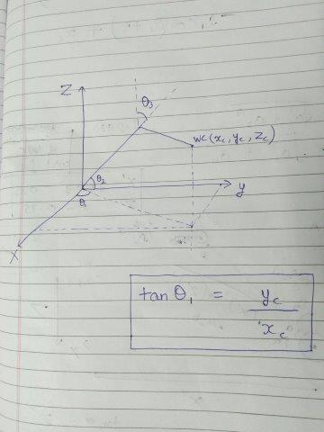
theta1 = atan2( yc , xc)

where yx and xc are coordinates of the WC.

For calculating we look in the Z-X frame of reference.

Theta2

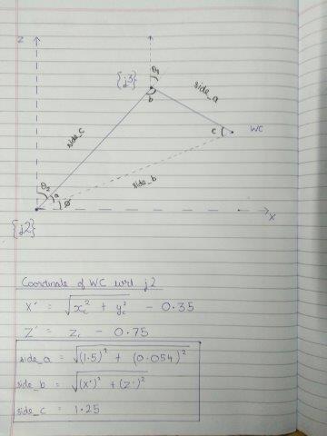
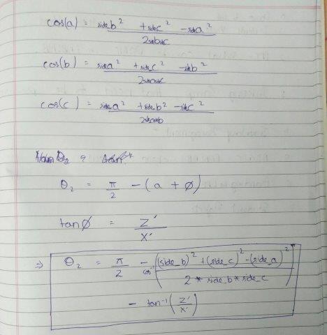
For calculating theta2, because the side_a, side_b and side_c is known, cosine rule is used to find the angles of the triangle in the figure below.

theta2 = pi / 2  -  angle_a - phi

Theta3

The joint angle theta3 is also calculated using the angles found using the cosine rule.

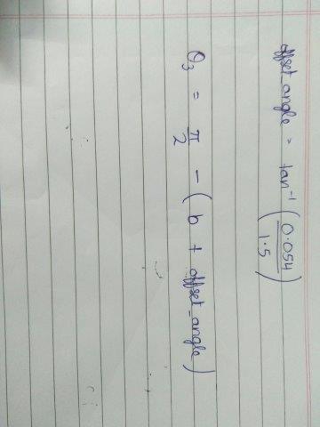
theta3 = pi / 2 - offset_angle - angle_b

angle_a , angle_b as the figure.

offset_angle is introduced because the centre points of j3 and j4, j5 and j6 are not collinear.

For calculating theta4, theta5 and theta6

These joint angles can be calculated by observing the symbolic representation of R3_6 and manipulating its elements. It can out to be:

R3_6 = Matrix([
        [-sin(q4)*sin(q6) + cos(q4)*cos(q5)*cos(q6), -sin(q4)*cos(q6) - sin(q6)*cos(q4)*cos(q5), -sin(q5)*cos(q4)],
        [                           sin(q5)*cos(q6),                           -sin(q5)*sin(q6),          cos(q5)],
        [-sin(q4)*cos(q5)*cos(q6) - sin(q6)*cos(q4),  sin(q4)*sin(q6)*cos(q5) - cos(q4)*cos(q6),  sin(q4)*sin(q5)]])

theta4

tan(theta4) = R3_6[2,2] / -R3_6[0,2]

theta5

tan(theta5) = sqrt(R3_6[0, 2] * R3_6[0, 2] + R3_6[2,2] * R3_6[2,2]) / R3_6[1,2])

theta6

tan(theta6) = -R3_6[1,1] / R3_6[1,0]

After finding out these angles, they were published to the RViz which moves the robotics arm KR210 also simulated in the Gazebo environment.

Results

The inverse kinematics solution refers to finding the angles that the joints of the robotic arm need to be at so that the the end effector is at the desired position with the desired orientation. This can also be called the desired pose(position + orientation). This is a harder problem compared to forward kinematics (using joint angles to find the position and orientation of the end effector) and multiple solutions maybe present(in the dexterous workspace).

The inverse kinematics solutions were calculated in approximately 1 second per solution for the points in the path planned by RViz. For real time applications, this should be in the order of milliseconds.

Improvements

This project can be improved by making a program that can produce closed-form inverse kinematics solutions automagically from the URDF file of the robot. Something like ik_fast. Shifting to compiled languages will also reduce time to calculate the IK solutions.

Where it might Fail

This will fail to calculate solutions if the point to be reached is at a greater distance than the workspace of the robot, although in real cases extenders might be used at the cost of payload capacity. Mobile manipulators is also another option for pick and placement of far away objects.