Dual Layer Neural network and PCA optimized for a ranking engine.

2 Layer Neural network using keras and python for a recommendation engine.

Lesson 1, ipynb notebook, flattened to PDF:

https://github.com/sentientmachine/DualLayerNN_and_PCA_for_recommendation_system/blob/master/Day1_lesson1_keras_2_layer_alg.pdf

Reproduction of Lesson1's work:

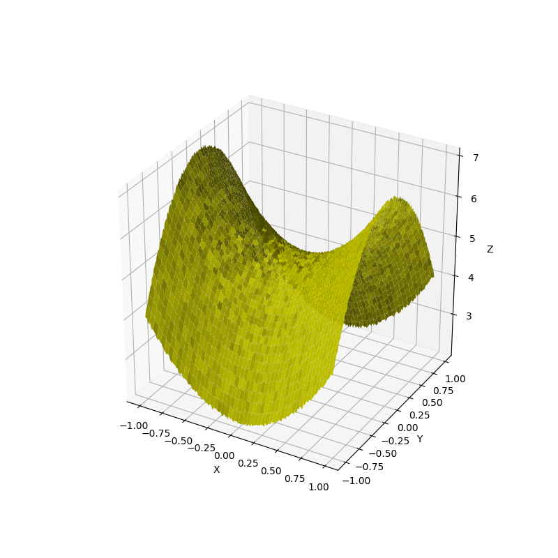
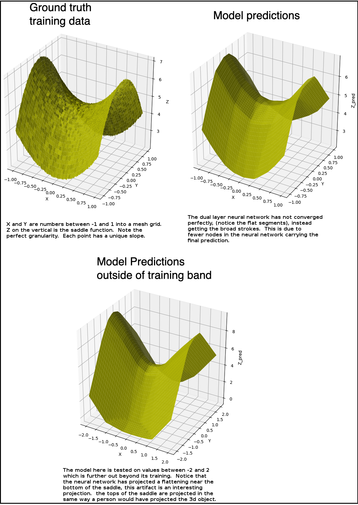
To prove that our machine learning engine is working, Demo of learning a Noisy Saddle Function => z=2*x*x-3*y*y+5+e

Dataset is MovieLens DataSet: https://grouplens.org/datasets/movielens

MovieLens data has been downloaded in this git repo:

ratings.csv
users.csv
items.csv

Python code reproduces the work:

#!/usr/bin/python
# -*- coding: utf-8 -*-

#Basics of Deep Learning

#Load Libraries
import numpy as np
import pandas as pd

#Load libraries for Visualisation.
import matplotlib.pyplot as plt
import altair as alt

#disable warnings for tensorflow, and add library tensorflow, 
#tensorflow is still early-alpha-software and a big crybaby
import warnings
warnings.filterwarnings('ignore')
import tensorflow as tf
import recoflow
from recoflow.vis import Vis3d
warnings.resetwarnings()

#create some ranges of data for X and Y across 2 dimensions
x = np.arange(start = -1, stop = 1, step = 0.01)
y = np.arange(-1, 1, 0.01)

#Make a meshgrid that creates a 2d plane with it.
X, Y = np.meshgrid(x,y)
c = np.ones([200, 200])
e = np.random.rand(200, 200)*0.1

#lift the plane into the Z dimension to create a saddle 3d shape
Z = 2*X*X - 3*Y*Y + 5*c + e

#prepare and save the image
fig = plt.figure(figsize=(8,8))
ax = fig.add_subplot(111, projection='3d')
ax.plot_surface(X, Y, Z, color='y')
ax.set_xlabel('X')
ax.set_ylabel('Y')
ax.set_zlabel('Z')

#save out the image
plt.savefig('saddle.png')

X and Y are the input training, and Z is the prediction, the result of the Z saddle function.

The above saddle is an arbitrary target Z, train the model to learn it:

#Using Deep Learning
#Step 0: Load Libraries

from keras.models import Model
from keras.layers import Dense, Input, Concatenate


#Step 1: Design the Learning Architecture, model definition
def deep_learning_model():

    # Get the input
    x_input = Input(shape=[1], name="X")
    y_input = Input(shape=[1], name="Y")

    # Concatenate the input
    xy_input = Concatenate(name="Concat")([x_input, y_input])

    # Create Transform functions
    Dense_1 = Dense(32, activation="relu", name="Dense1")(xy_input)
    Dense_2 = Dense(4, activation="relu", name="Dense2")(Dense_1)

    # Create the Output
    z_output = Dense(1, name="Z")(Dense_2)

    # Create the Model
    model = Model([x_input, y_input], z_output, name="Saddle")

    # Compile the Model
    model.compile(loss="mean_squared_error", optimizer="sgd")

    return model

model = deep_learning_model()
model.summary()


#is this broke?
#from keras.utils import plot_model
#plot_model(model, show_layer_names=True, show_shapes=True)

#Step 2 learn the weights:
input_x = X.reshape(-1)
input_y = Y.reshape(-1)
output_z = Z.reshape(-1)
X.shape, Y.shape, Z.shape

input_x.shape, input_y.shape, output_z.shape

df = pd.DataFrame({"X": input_x, "Y": input_y, "Z": output_z})
df.head()

#fit the model
output = model.fit( [input_x, input_y], output_z, epochs=10,
               validation_split=0.2, shuffle=True, verbose=1)

#Step 4: Evaluate Model Performance
from recoflow.vis import MetricsVis
df = pd.DataFrame(output.history)
df.reset_index()
df["batch"] = df.index + 1
df = df.melt("batch", var_name="name")
df["val"] = df.name.str.startswith("val")
df["type"] = df["val"]
df["metrics"] = df["val"]
df.loc[df.val == False, "type"] = "training"
df.loc[df.val == True, "type"] = "validation"
df.loc[df.val == False, "metrics"] = df.name
df.loc[df.val == True, "metrics"] = df.name.str.split("val_", expand=True)[1]
df = df.drop(["name", "val"], axis=1)
base = alt.Chart().encode(
    x = "batch:Q",
    y = "value:Q",
    color = "type"
).properties(width = 300, height = 300)
layers = base.mark_circle(size = 50).encode(tooltip = ["batch", "value"]) + base.mark_line()
chart = layers.facet(column='metrics:N', data=df).resolve_scale(y='independent')
chart.save('eval_model_performance.png')

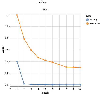
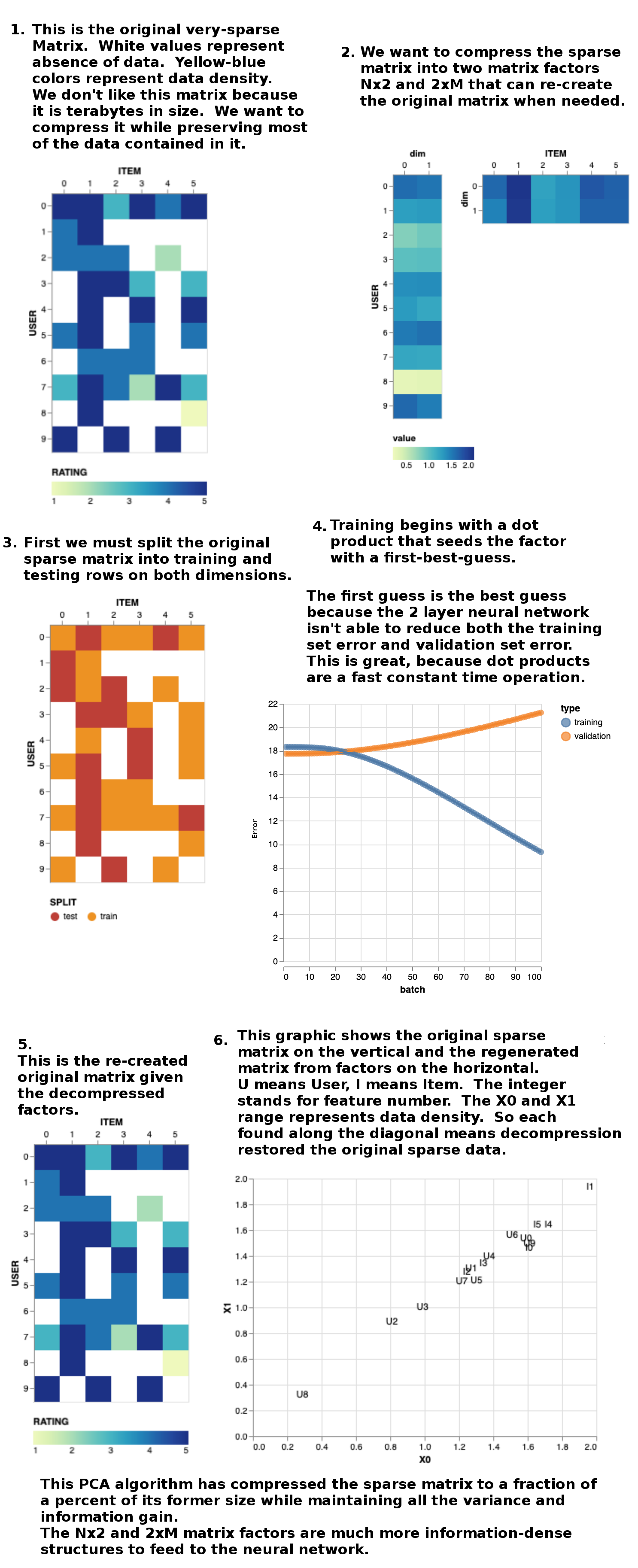
The algorithm splits the X and Y into training and testing sets and trains upon the training set and decreases the error between the predicted target and the correct target. The model learns the training data immediately, and slowly gets closer to perfection in the testing data.

#Step 5: Make a Prediction
Z_pred = model.predict([input_x, input_y]).reshape(200,200)

#prepare and save the image
fig = plt.figure(figsize=(8,8))
ax = fig.add_subplot(111, projection='3d')
ax.plot_surface(X, Y, Z_pred, color='y')
ax.set_xlabel('X')
ax.set_ylabel('Y')
ax.set_zlabel('Z_pred')

#save out the image
plt.savefig('saddle_learned.png')

Moneyshot

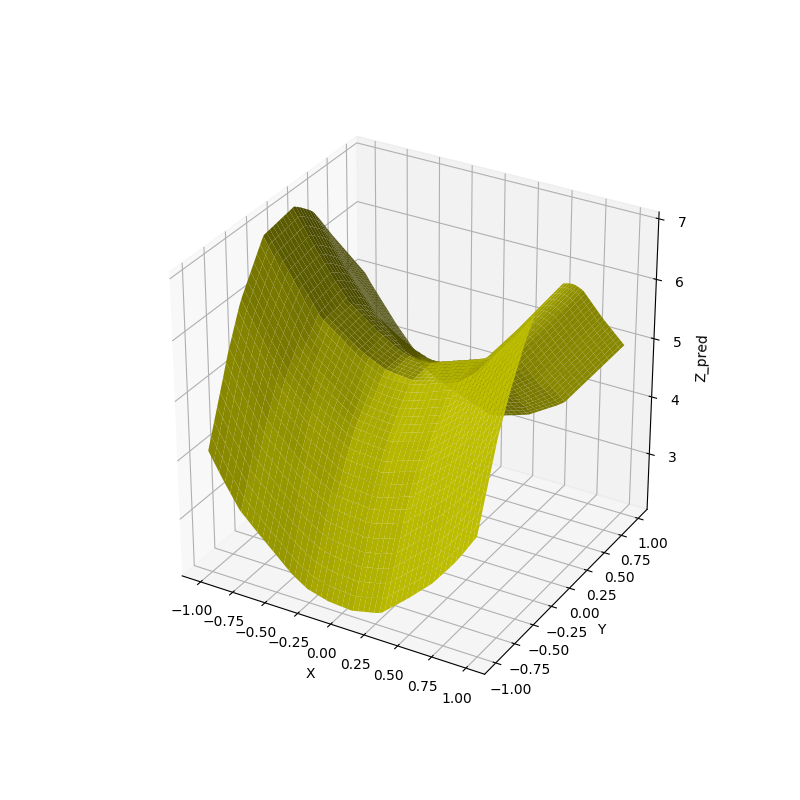
The previous image shows that the dual layer neural network has correctly reproduced the prediction Z axis from every input X/Y. But if you can read the code, you would protest we could have achieved the same objective with a one to one hashmap! But to that we say hashmaps don't generalize, so lets show you how ours generalizes.

#Step 5b: Make a Prediction out of band, how are we looking?

#create some ranges of data for X and Y across 2 dimensions
x = np.arange(start = -2, stop = 2, step = 0.02)
y = np.arange(-2, 2, 0.02)

#Make a meshgrid that creates a 2d plane with it.
X, Y = np.meshgrid(x,y)

input_x = X.reshape(-1)
input_y = Y.reshape(-1)

Z_pred = model.predict([input_x, input_y]).reshape(200,200)

#prepare and save the image
fig = plt.figure(figsize=(8,8))
ax = fig.add_subplot(111, projection='3d')
ax.plot_surface(X, Y, Z_pred, color='y')
ax.set_xlabel('X')
ax.set_ylabel('Y')
ax.set_zlabel('Z_pred')

#save out the image
plt.savefig('saddle_learned_out_of_band.png')

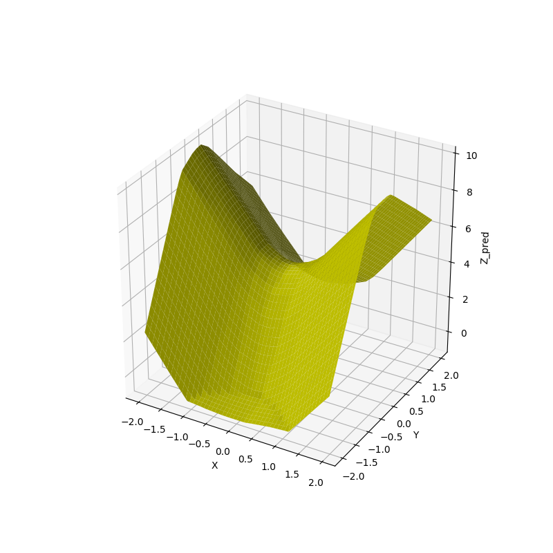
Notice the X and Y axis has been increased out of the training band from -2 to 2, rather than just the training data -1 to 1. This provides some evidence that our model is correctly flinging the generalized projection area into visably pleasing directions.

The three side by side:

Day 1 Lesson 1 - doing PCA Principal Components Analysis via matrix factorization to maximize variance and minimize set size, for generalization.

https://github.com/sentientmachine/DualLayerNN_and_PCA_for_recommendation_system/blob/master/Day1_lesson2_pca_matrix_factorization.pdf

Tensorflow Tutorial basic Text Classification:

ipynb notebook flattened to PDF:

https://github.com/sentientmachine/DualLayerNN_and_PCA_for_recommendation_system/blob/master/tensorflow_tutorial_basic_text_classification.pdf

Day2 deep models for ranking

ipynb notebook flattened to PDF:

https://github.com/sentientmachine/DualLayerNN_and_PCA_for_recommendation_system/blob/master/day2_lesson4_deepmodels_ranking.pdf

Reproduction

#!/usr/bin/python
# -*- coding: utf-8 -*-

import warnings
warnings.filterwarnings('ignore')

#import recoflow
import numpy as np
import pandas as pd
from recoflow.preprocessing import EncodeUserItem, StratifiedSplit

import matplotlib.image as mpimg
import PIL
import matplotlib.pyplot as plt

warnings.resetwarnings()
ratings = pd.read_csv("ratings.csv")
users = pd.read_csv("users.csv")
items = pd.read_csv("items.csv")


# Encoding the data
interaction, n_users, n_items, user_encoder, item_encoder = EncodeUserItem(ratings,
                                                                          "user_id",
                                                                          "movie_id",
                                                                          "rating",
                                                                          "unix_timestamp")


train, test = StratifiedSplit(interaction, [0.8, 0.2])
train.shape, test.shape
#((80000, 7), (20000, 7))
min_rating = interaction.RATING.min()
max_rating = interaction.RATING.max()
min_rating, max_rating
#(1, 5)

# Model - Deep Factorisation
from keras.models import Model
from keras.layers import Embedding, Input, Dot, Add, Activation, Lambda, Concatenate, Dense, Flatten, Dropout
from keras.regularizers import l2
from keras.optimizers import Adam


def DeepMF(n_users, n_items, n_factors, min_rating, max_rating):

    # Item Layer
    item_input = Input(shape=[1], name='Item')
    item_embedding = Embedding(n_items, n_factors, embeddings_regularizer=l2(1e-6),
                               embeddings_initializer="glorot_normal",
                               name='ItemEmbedding')(item_input)
    item_vec = Flatten(name='FlattenItemE')(item_embedding)

    # Item Bias
    item_bias = Embedding(n_items, 1, embeddings_regularizer=l2(1e-6),
                               embeddings_initializer="glorot_normal",
                          name='ItemBias')(item_input)
    item_bias_vec = Flatten(name='FlattenItemBiasE')(item_bias)

    # User Layer
    user_input = Input(shape=[1], name='User')
    user_embedding = Embedding(n_users, n_factors, embeddings_regularizer=l2(1e-6),
                              embeddings_initializer="glorot_normal",
                               name='UserEmbedding')(user_input)
    user_vec = Flatten(name='FlattenUserE')(user_embedding)

    # User Bias
    user_bias = Embedding(n_users, 1, embeddings_regularizer=l2(1e-6),
                              embeddings_initializer="glorot_normal",
                              name='UserBias')(user_input)
    user_bias_vec = Flatten(name='FlattenUserBiasE')(user_bias)

    # Concatenation of Item and User & then Add Bias
    Concat = Concatenate(name="Concat")([item_vec, user_vec])
    ConcatDrop = Dropout(0.5)(Concat)

    # Use the Dense layer for non-linear interaction learning
    Dense_1 = Dense(32, name="Dense1", activation="relu")(ConcatDrop)
    Dense_1_Drop = Dropout(0.5)(Dense_1)
    Dense_2 = Dense(1, name="Dense2")(Dense_1_Drop)

    # Add the Bias
    AddBias = Add(name="AddBias")([Dense_2, item_bias_vec, user_bias_vec])

    # Scaling for each user
    y = Activation('sigmoid')(AddBias)
    rating_output = Lambda(lambda x: x * (max_rating - min_rating) + min_rating)(y)

    # Model Creation
    model = Model([user_input, item_input], rating_output, name="DeepFM")

    # Compile Model
    model.compile(loss='mean_squared_error', optimizer=Adam(lr=0.001))

    return model



n_factors = 40
model = DeepMF(n_users, n_items, n_factors, min_rating, max_rating)

from keras.utils import plot_model
plot_model(model, show_layer_names=True, show_shapes=True, to_file='lesson4_model.png')

model.summary()


output = model.fit([train.USER, train.ITEM], train.RATING,
                  batch_size=32, epochs=5, verbose=1,
                  validation_data=([test.USER, test.ITEM], test.RATING))


from recoflow.vis import MetricsVis
MetricsVis(output.history)


from recoflow.recommend import GetPredictions

#%%time
predictions = GetPredictions(model, interaction)
#CPU times: user 33.2 s, sys: 4.01 s, total: 37.3 s
#Wall time: 23.7 s
predictions.shape
#(1586126, 3)
from recoflow.metrics import RatingMetrics
RatingMetrics(test, predictions)

from recoflow.recommend import ItemEmbedding, UserEmbedding
item_embedding = ItemEmbedding(model, "ItemEmbedding")
user_embedding = UserEmbedding(model, "UserEmbedding")
#Getting Recommendation

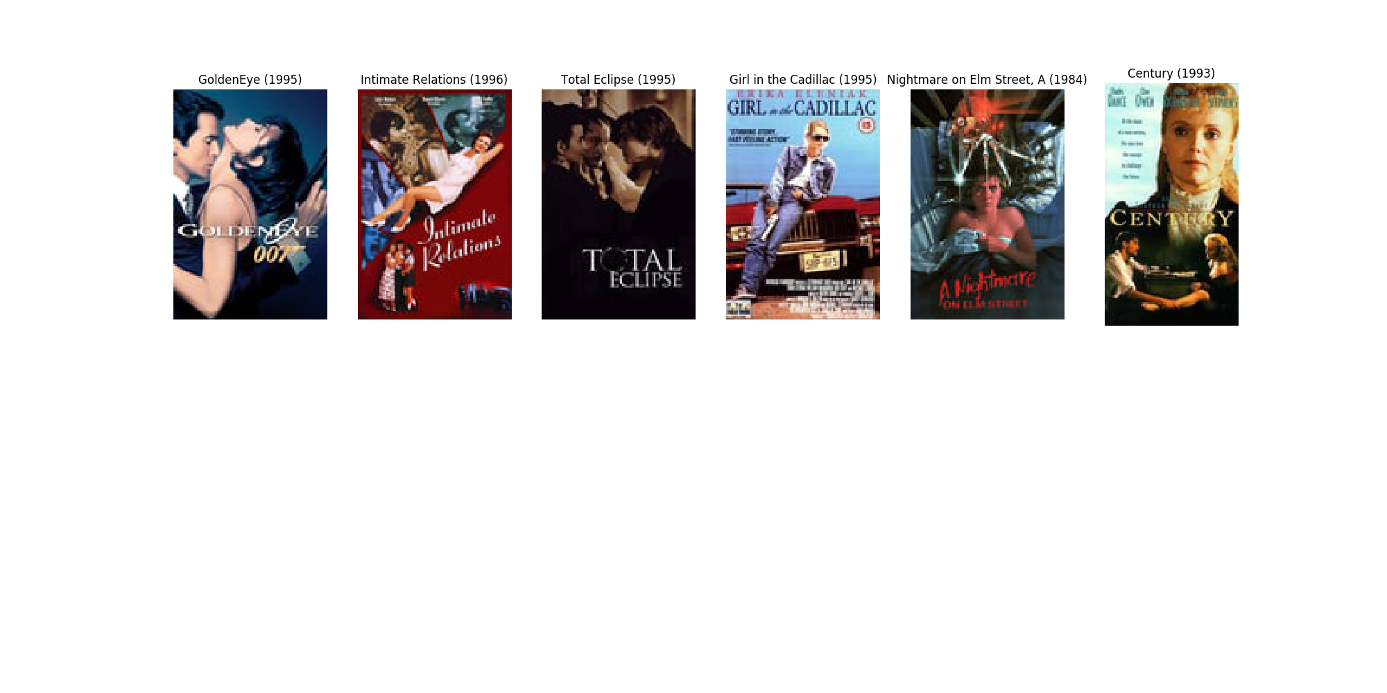
#Given an Item, what are the similiar items?
#Given a User, what items should I recommend?
from recoflow.recommend import GetSimilar, ShowSimilarItems
similar_items = GetSimilar(item_embedding, k=5, metric="euclidean")
similar_items

#ShowSimilarItems(1, similar_items, item_encoder, items, image_path='/tf/notebooks/data/data/posters/')
item_index = 1
item_similar_indices = similar_items
image_path='./posters/'

movie_title = items.iloc[0].title
s = item_similar_indices[item_index]
movie_ids = item_encoder.inverse_transform(s)
images = []
titles = []
for movie_id in movie_ids:
    img_path = image_path + str(movie_id) + '.jpg'
    images.append(mpimg.imread(img_path))
    title = items[items.movie_id == movie_id].title.tolist()[0]
    titles.append(title)

plt.figure(figsize=(20,10))
columns = 6
for i, image in enumerate(images):
    plt.subplot(len(images) / columns + 1, columns, i + 1)
    plt.axis('off')
    plt.imshow(image)
    plt.title(titles[i])

plt.savefig('lesson4_movie_titles.png')

Top Ranked Titles for our User.

from recoflow.recommend import GetRankingTopK
#Ranking Top K

#Get all the predictions for all users
#Remove all the items the user has already seen (train)
#Sort the remaining data by predicted ratings
#Cut-off at K
#%%time
ranking_topk = GetRankingTopK(model, interaction, train, k=5)
#CPU times: user 36.2 s, sys: 4.13 s, total: 40.3 s
#Wall time: 26.8 s
n_users * 5
#4715
ranking_topk.shape
#(4715, 4)
ranking_topk.head()


from recoflow.models import NeuralCollaborativeFiltering
ncf = NeuralCollaborativeFiltering(n_users, n_items, n_factors, min_rating, max_rating)
plot_model(ncf, show_layer_names=True, show_shapes=True)