PACT is a plug-in for EEGLAB. PACT stands for (cross-frequency) Phase-Amplitude Coupling Toolbox. See the github repository at https://github.com/sccn/PACT to submit bug reports or modify the codebase.
PACT was initially developed for analyzing electrocorticographic (ECoG) data. The applicability of using PACT on scalp-recorded EEG relies on the manner in which highest-amplitude sampling (HAS) is utilized. For more information, please refer to the next section. The current version of PACT supports event-related data analysis.
In the field of epileptology, it is well-established that ECoG data reveals the presence of transient bursts with high amplitude, which are associated with epileptogenesis. These bursts are commonly referred to as high-frequency oscillations (HFOs). Various algorithms have been developed to detect HFOs. However, some neurologists realized that HFO's sensitivity was limited. So they considered that pathological HFO may show characteristic coupling with low-frequency phase. Thus, they hypothesized that detecting HFOs then evaluating their PAC patterns should improve sensitivity. This is the basic motivation of PACT that can quantify PAC of HFOs. Thus, the PACT first identifies potential HFO candidates by applying a straightforward amplitude threshold. Afterward, PAC is computed using only the selected data points. When HAS is set to 100%, it calculates the original Canolty's modulation index (MI).
The simple answer is yes, as long as you are knowledgeable about the process.
The more detailed answer is that it depends on how you process data. One key difference between ECoG and scalp-recorded EEG is that the latter is prone to contamination from artifacts such as blinks, eye movements, muscle potentials, and line noise at frequencies like 50Hz or 60Hz. Some of these artifacts have a dominant power distribution in higher frequency ranges, including beta and gamma.
To effectively apply PACT to scalp-recorded EEG data, it is recommended to select data with minimal artifacts. For instance, blinks often produce phase-amplitude coupled artifacts. Users should be familiar with the basic qualities of signals and artifacts, and exercise caution when using PACT. Additionally, it is advised to systematically vary HAS values to observe how it affects the results.
Always remember that while selecting high-amplitudes is effective for identifying HFOs in ECoG, it also introduces potential bias towards different types of artifacts in scalp-recorded EEG data.
Miyakoshi M, Nariai H, Rajaraman RR, Bernardo D, Shrey DW, Lopour BA, Sim MS, Staba RJ, Hussain SA. (2021). Automated preprocessing and phase-amplitude coupling analysis of scalp EEG discriminates infantile spasms from controls during wakefulness. Epilepsy Res. 178:106809.
In this paper, HAS of 2% is used. The relevant description in the method section is cited below.
Data points with gamma amplitude larger than the 98th percentile were marked as high amplitude samples (HAS)
However, this does not mean 2% is the generally recommended value for all the applications. It serves one of the potential anchor points which showed successful results. I recommend we stick to familiar values like 5% (0.05), 1% (0.01), etc. that are widely accepted values in the application of inferential statistics. As you parametrically change the HAS values from small to large values, you might find non-linear responses. You should determine what you are sensing there, whether it is an artifact (blinks, saccades, etc.) or brain signals (genuine HFO-PAC in the EEG signals).
In preparatory exploration, you may run a brute-force computation of PAC for all combinations of low-frequency oscillation (LFO) and highest-amplitude sampling (HAS) center frequencies. This computation may take a long time depending on the frequency resolution and bandwidth you specify. To compute each PAC value for a channel frequency-by-frequency combination, PACT performs the following steps:
1. Band-pass filter the data to extract HFO and LFO signals.
2. Hilbert transform the HFO signal to extract a time series of instantaneous amplitudes.
3. Hilbert transform the LFO signal to extract a time series of instantaneous phases.
4. (Highest-Amplitude Sampling, HAS): apply a threshold to select the N% highest HFO amplitudes. Obtain the HAS index from this.
5. For LFO phase, apply HAS index.
6. Combine HAS-indexed HFO and LFO indices into complex-valued phasors.
7. Compute the Modulation Index (Canotly et al., 2006) for the collection of HAS phasors constructed above.
8. Generate a collection of surrogate data by circularly permuting the phase time-series relative to the amplitude series.
9. Compute a surrogate set of Modulation Indices for which the null hypothesis should hold and determine a statistical threshold from their distribution.
10. Perform multiple comparison corrections based on the number of channels for which you are estimating PAC significance.
Note: To compute and perform statistics on the Mean Resultant Vector Length, PACT uses CircStat (Berens, 2009). To compute phase-sorted amplitude statistics, PACT uses K-S and Chi-square tests.
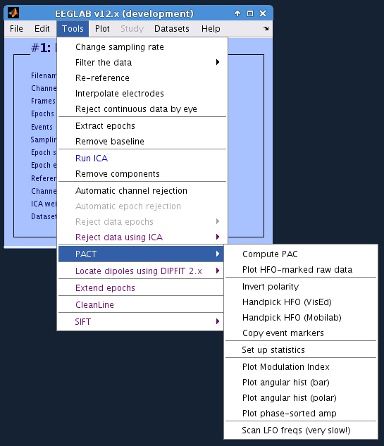
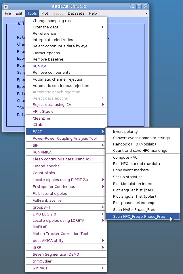
Figure 1. PACT Seen from EEGLAB main GUI.
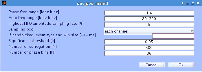
Figure 2. Main GUI
When successfully installed, the item 'PACT' should appear under 'Tools' (Figure 1). Currently it has 12 menus.
- Compute PAC: This launches the main GUI (Figure 2). When press ok,
computation starts. When it done, statistics set up window pops up
(described later).
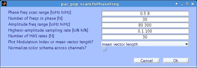
- Phase freq range [lohz hihz]
- Amp freq range [lohz hihz]
- Highest amplitude sampling rate [%]
- Sampling pool: This is for the experimental purpose. Always choose 'Each channel'.
- If handpicked, event type and win size [+/- ms]: If you want to run the analysis using the data around event markers generated by either VidEd or MoBILAB, use this.
- Significance threshold [p]
- Number of surrogation [N]: This determines how many data points you want to generate surrogate data that represents for distribution of null hypothesis.
- Number of phase bins [N]: This affects sensitivity of circular statistics. Don't use too extremely large value (e.g. >100).
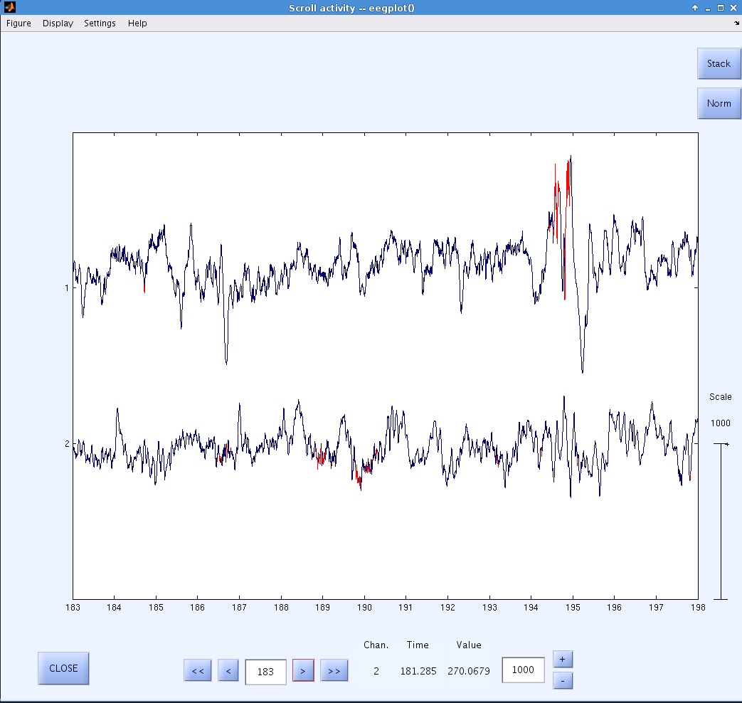
Figure 3. Detected HFOs (shown in red)
- Plot HFO-marked Raw data: This plot looks like Figure 3.
- Invert polarity: This is to invert EEG polarity by simply multiplying -1 to all the data.
The function described in the following section is depricated (works only in Matlab 2013 or older)
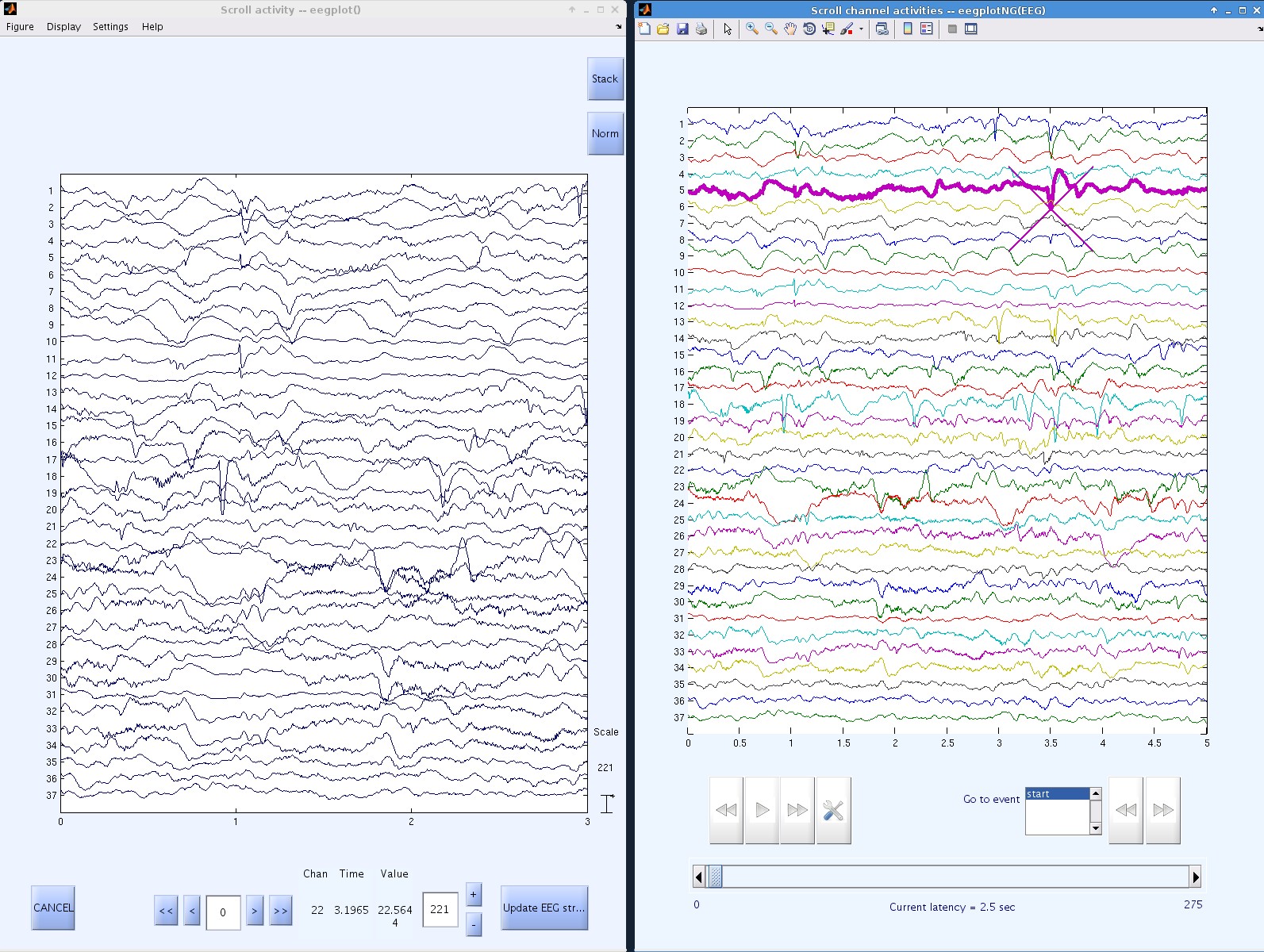
Figure 4. Manually marking HFOs. Left, using VisEd. Right, using customized MoBILAB plots
Handpick HFO(VisEd): This plot looks like Figure 4 left. You canchoose the marking point by mouse click. For detailed explanationhow to use this VisEd, see VisEd help.Handpick HFO(Mobilab): This plot looks like Figure 4 left.Similarly, you can choose the marking point by mouse click. Usewhichever suit you.Copy event markers: This is to copy event markers from dataset 1 to dataset 2.
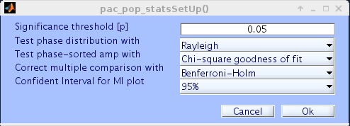
Figure 5. Statistics set up
- Set up statistics: This shows a GUI that look like Figure 5.
- Plot Modulation Index: This shows a plot that look like Figure 7/8 top right.
- Plot Angular hist (bar)
- Plot Angular hist (polar): This shows a plot that look like Figure 7/8 bottom left.
- Plot phase-sorted amp: This shows a plot that look like Figure 7/8 bottom left. Each bar represents mean amplitude of each phase bin.
Figure 6. Scanning parameter space consists of LFO phase frequencies and HAS rates
- Scan LFO freqs (very slow!): This pops up GUI like Figure 6. Start with N = 10 or around, and HAS rate of 0.3-10. Color normalization should be used when plotting Mean Resultant Vector Length.
1. LFO-HAS parameter space scan results (combination of LFO phase frequencies and HAS rates; the measure used may be either Mean Resultant Vector Length or Modulation Index.
2. Using Modulation Index with a confidence interval of 95% or 99%.
3a. Angular histogram displayed in a polar plot using Mean Resultant Vector Length.
3b. Angular histogram in a rectangular plot with phase unwrapped on the x-axis.
4. Bar graphs of LFO phase-sorted HFO-amplitudes.
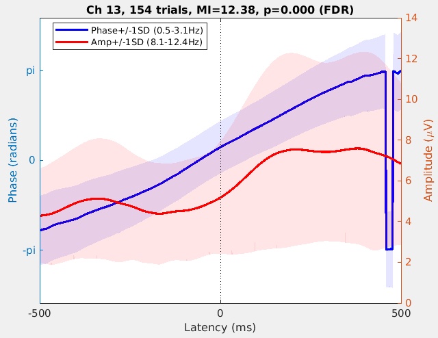
5. (When event-related PAC is selected) Time-domain phase-amplitude time series. See below.
Note that the number of phase bins in Figures 3a and 3b is determined by user input and affects the results of the circular statistics.
These plots show examples in which PACT was applied to electrocorticographic data for which a neurologist judged the channel( Ch) 1 signal to be pathological and the Ch2 signal to be normal.
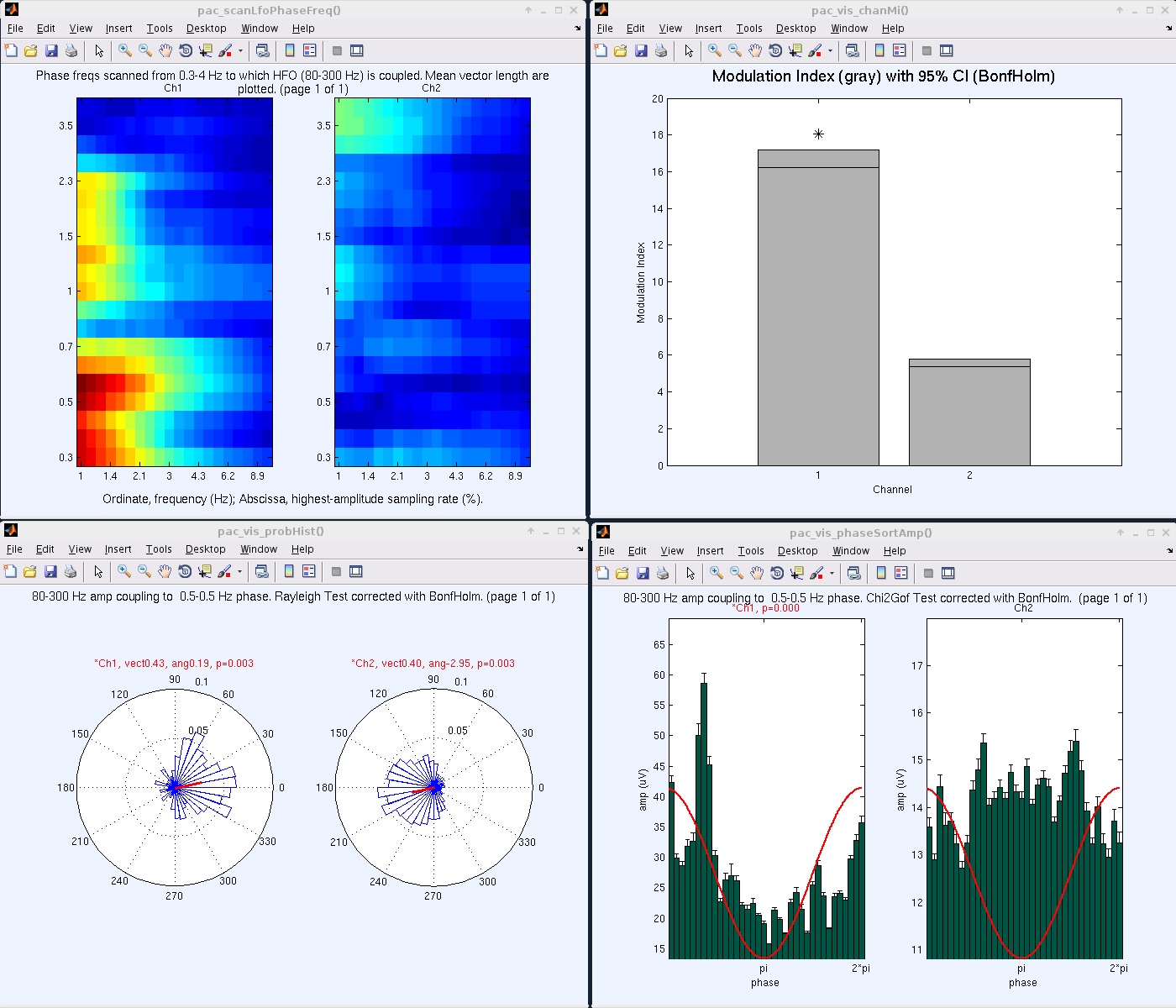
First, exploratory LFO frequency scans were performed (Figures 7 and 8, top left; they are the same). We needed to run PACT several times, adjusting parameters; the result that showed the difference most clearly is plotted here. Mean Resultant Vector Length was chosen as the dependent variable, since it is naturally normalized from 0 to 1 and is therefore convenient for comparisons across channels. This plot shows two noticeable clusters of interest that showed differences between Ch1 and Ch2:.One is (LFO 0.5 Hz, HAS 3%,) the other (LFO 1.5 Hz, HAS 1.5%). We decided to run analysis for both combinations of parameters. Statistical significance level was set to 1% with Bonferroni-Holm correction (Note: here, since we have only 2 items to compare, B-H is the same as Bonferroni).
Figure 7. LFO 0.5Hz, HAS 3%, p < 0.01, CI 95%. Top left, LFO-HAS parameter space scan results. Top right, Modulation Index. Bottom left, Mean Resultant Vector Length. Bottom right, phase-sorted HFO amplitudes
Figure 7 shows the result of choosing parameters (LFO0.5 Hz, HAS 3%). The Modulation Index for Ch1 is larger than that for Ch2. Only the Ch1 value reached statistical significance (Figure 7, top right; a horizontal bar in the graph shows the 95% confidence interval). By Mean Resultant Vector length, both channel signals exhibited showed phase concentrations, though their preferred phases were different -- almost opposite (Figure 7, bottom left). Phase-sorted HFO amplitude also indicated that Ch1 has a preferred phase, and the Ch1 amplitude distribution over phase bins deviates significantly from uniform, whereas Ch2 does not show this effect (Figure 7, bottom right). Note also the large difference in amplitude scales.
Figure 8. LFO 1.5Hz, HAS 1.5%, p < 0.01, CI 95%. Top right, Modulation Index. Bottom left, Mean Resultant Vector Length. Bottom right, Phase-sorted HFO amplitude. Note that the Ch1 Modulation Index is much larger than the confidence interval compared to Figure 7
Figure 8 shows the result of choosing the parameters (LFO 1.5 Hz, HAS 1.5%). Modulation Index, Mean Resultant Vector length, and Phase-sorted HFO amplitude all showed similar properties to the results shown in Figure 7. However, note that the Ch1 Modulation Index is much larger than its confidence interval level; probably this combination of parameters better fits the pathological pattern in this channel signal.
http://sccn.ucsd.edu/wiki/Plugin_list_process
The 'Handpick HFO' menu does not work with newer Matlab versions, which no longer support the graphics.cursorbar object. To use this function, use Matlab 2013 or older as a workaround.
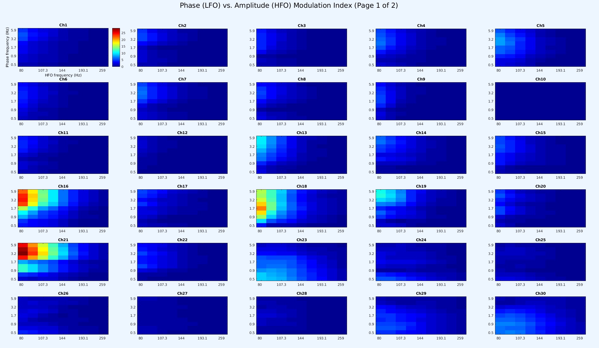
In calculating phase-amplitude coupling, a typical problem is how to determine the target frequencies in both phase and amplitude. To perform it simply, in ver.0.30 I implemented a function to generate phase-amplitude frequency-by-frequency grid plot. If you need to reduce the number of channel, do so by using EEGLAB GUI beforehand. Otherwise, this frequency scan process does not need any preprocessing by PACT, it does the job itself. One extra parameter you have to choose is highest amplitude sampling (HAS) rate, which specifies the right-tail cutoff for the amplitude distribution for each channel. Note that this is only picking up the highest amplitude after high-frequency band-pass filter, so if there is artifact with high-frequency (or broadband), HAS will pick it up. In this case, you would want to clean the data using EEGLAB function before performing this analysis.
In the example below, one can easily find that Ch21 showed the strongest PAC between 3-Hz phase and 80-Hz HFO amplitude, followed by Ch16. Ch18 also showed some PAC, but it coupled with 1.7 Hz instead of 3 Hz so this could be something different. If one chooses mean vector length to show instead of Canolty's modulation index (MI), it allows to evaluate the same measure without the effect of HFO amplitude. The calculated values are stored under EEG.pacScan.
- In the plot above, confirm that the peak PAC value is observed at Ch21, phase 3.2-Hz, ampltiude 80-Hz.
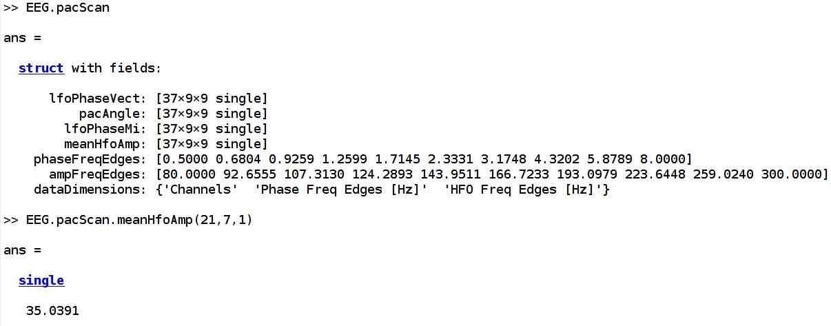
- Type 'EEG.pacScan' in the command line. Among the variables, find 'meanHfoAmp' This is mean HFO amplitude in microVolt. If you are not sure about dimensions, see 'dataDimensions'. We know our channel and freq-freq window of interest, which are 21, 3.2 Hz, 80 Hz, respectively. Based on these parameters of interest, we obtain indices for these parameters: 21 for the channel order, 7 for the phase freq (see 'phaseFreqEdge'--3.2Hz is between the 7th and 8th edges, so we select 7), and 1 for the HFO freq.
- We enter EEG.pacScan.meanHfoAmp(21,7,1) in the command window. It returned '35.0391' which mean the mean HFO amplitude during the selected HFO frames was 35.0391 microVolt.
Please post bugs and suggestions to the EEGLAB mailing list.
http://www.ncbi.nlm.nih.gov/pubmed/24110429 Makoto Miyakoshi, Arnaud Delorme, Tim Mullen, Katsuaki Kojima, Scott Makeig, Eishi Asano. Automated detection of cross-frequency coupling in the electrocorticogram for clinical inspection. Conf Proc IEEE Eng Med Biol Soc.2013.3282-3285.
