NPLsizer

Python code to semi-automatically calculate the size of rectangular nanoplatelets from microscopy images.

Installation

Prerequisites

Python >= 3.8 is required for installation, along with the following Python packages.

Please note that I have tested the code only with Python 3.8 with the specific versions of the dependencies listed above inside parentheses, so make sure all the dependencies work if you are using a later version.

Installation using Conda

I recommend using the Conda Package Manager to install all the prerequisites. Make sure to use conda >= 22.11.

After installing conda, it is recommended to use a clean virtual environment for installing all the prerequisites. The code below creates a new environment myenv with python 3.8.

conda create -y -n myenv -c conda-forge python=3.8
conda activate myenv

[Optional] Sometime conda has difficulty in locating the appropriate set of compatible packages. It may help to change the default solver to libmamba.

conda update -n base conda
conda install -n base conda-libmamba-solver
conda config --set solver libmamba

Install most of the prerequisites. scikit-image and pillow should be automatically installed by conda as a dependency of some of these packages.

conda install -c conda-forge --override-channels numpy scipy napari pyqt magicgui opencv

Download a zip file of pyDM3reader from the website listed above and save it in your working directory.

pip install pyDM3reader-1.5.zip

Update everything.

conda update --all

User Guide

Before using the program, it may be helpful to gain some familiarity with the GUI features of the Napari viewer.

Starting the program

Download the source files and save them to a new directory. Open the terminal and navigate to the directory where you saved the source files.

Make sure that the conda environment where you installed all the packages earlier is activated. For example, if you installed the packages in myenv, type at the terminal

conda env list

You will see a list of existing environments with a * next to myenv. If this is not the case, please activate myenv thus

conda activate myenv

Note that if you launch a new shell, you may need to perform the activation process again.

Start the program from the command line

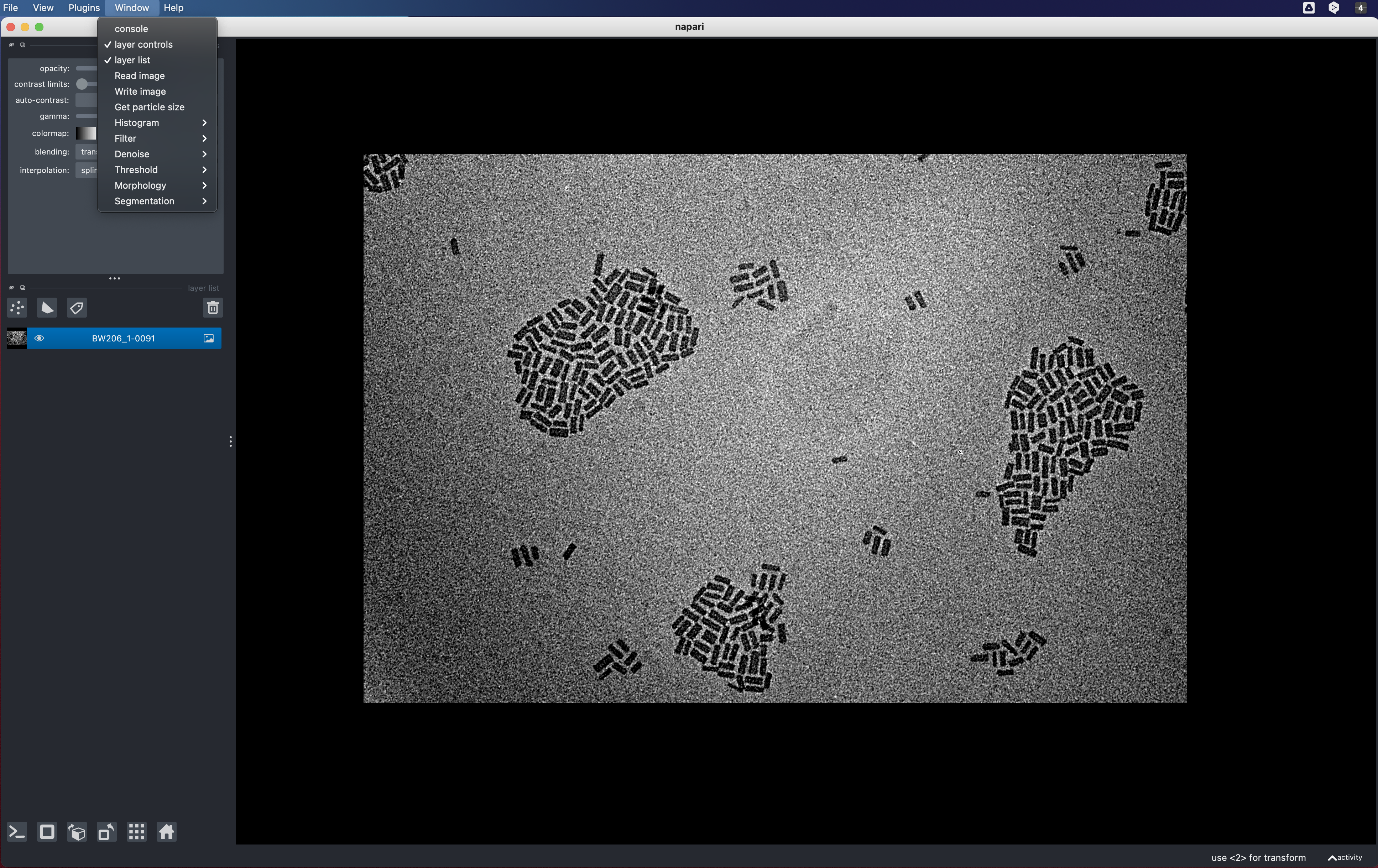
python NPLsizer.py

The Napari viewer window will launch. Almost all relevant functions are listed under the Window tab on the menubar of the main window.

Reading and writing images

Images to be analyzed are expected to be grayscale (array element data type int/float) or binary (data type bool). RGB images, if chosen, will be converted to grayscale.

To read an image, click on Window > Read image and enter/select the appropriate values for each field.

Any image format that can be read by scikit-image is acceptable. In addition, numpy .npy and .dm3 files can also be read. For .dm3 files, you may save its metadata in a separate file.

By default, the file name is used as the name of the image layer in the viewer, but you can supply a different name in the field Image layer name. Note that layer names are unique, so if you load an image with the same layer name as an existing layer, the existing layer will be overwritten.

To save/write an image, click on Window > Write image and enter/select the appropriate values for each field.

Output file format is determined from the file name extension. Any format that scikit-image can handle is allowed, in addition to .npy format. File output format cannot be .dm3.

Histogram manipulation

After loading an image, it is recommended to perform some histogram manipulation (Window > Histogram). The resulting output will be added as a new image layer. You may hide existing image layers to aid visibility. In case of adaptive histogram equalization (CLAHE), you may need to adjust the parameters. Note that after changing the parameters, if the output layer will be overwritten if you use the same name for the output layer. The grid view option of the viewer may help you visually decide on choosing the desired output. Feel free to delete any layers that you no longer need.

Filters

Several filters are available in the tabs Window > Filter and Window > Denoise. For each case, make sure that you choose the correct input image layer. You will need to play with the input parameters to decide what works for you. Note that for some parameter choices, the underlying functions may take a while to return the output. For details on each filter, please consult the appropriate documentation as listed below:

Thresholding

For global thresholding using Otsu's method, choose Window > Threshold > Threshold (see here for more details).

For adaptive thresholding, choose Window > Threshold > Adaptive Threshold (see here for more details on the parameters).

Note that the output of a thresholding operation is a binary array (data type bool).

Morphological operations

Several common morphological operations are listed in Windows > Morphology. Note that both inputs and outputs to these operations are binary images.

A useful workflow after thresholding is Window > Morphology > Remove Objects followed by Window > Morphology > Fill Holes. Remove Objects removes small foreground objects (in white) from a black background and Fill Holes fills small background holes (in black) with a white foreground region.

For both of these operations, I suggest that you run first without the shapes and labels parameters. Then, if there are still objects that you wish to remove, add a Shapes and/or Labels layer from the labels panel in the viewer. Draw the shapes around the regions to be removed. You can draw the labels as well and mark the labels as 1. All pixels within the shapes and those labeled as 1 will be marked as background, i.e., removed. A similar workflow applies for Fill Holes as well. Afterwords, delete the shape and label layers or alter them and run again.

Segmentation

The aim here is to identify rectangular regions of white foreground against a black background. First label the image (make sure to choose the right layer) using Window > Segmentation > Label.

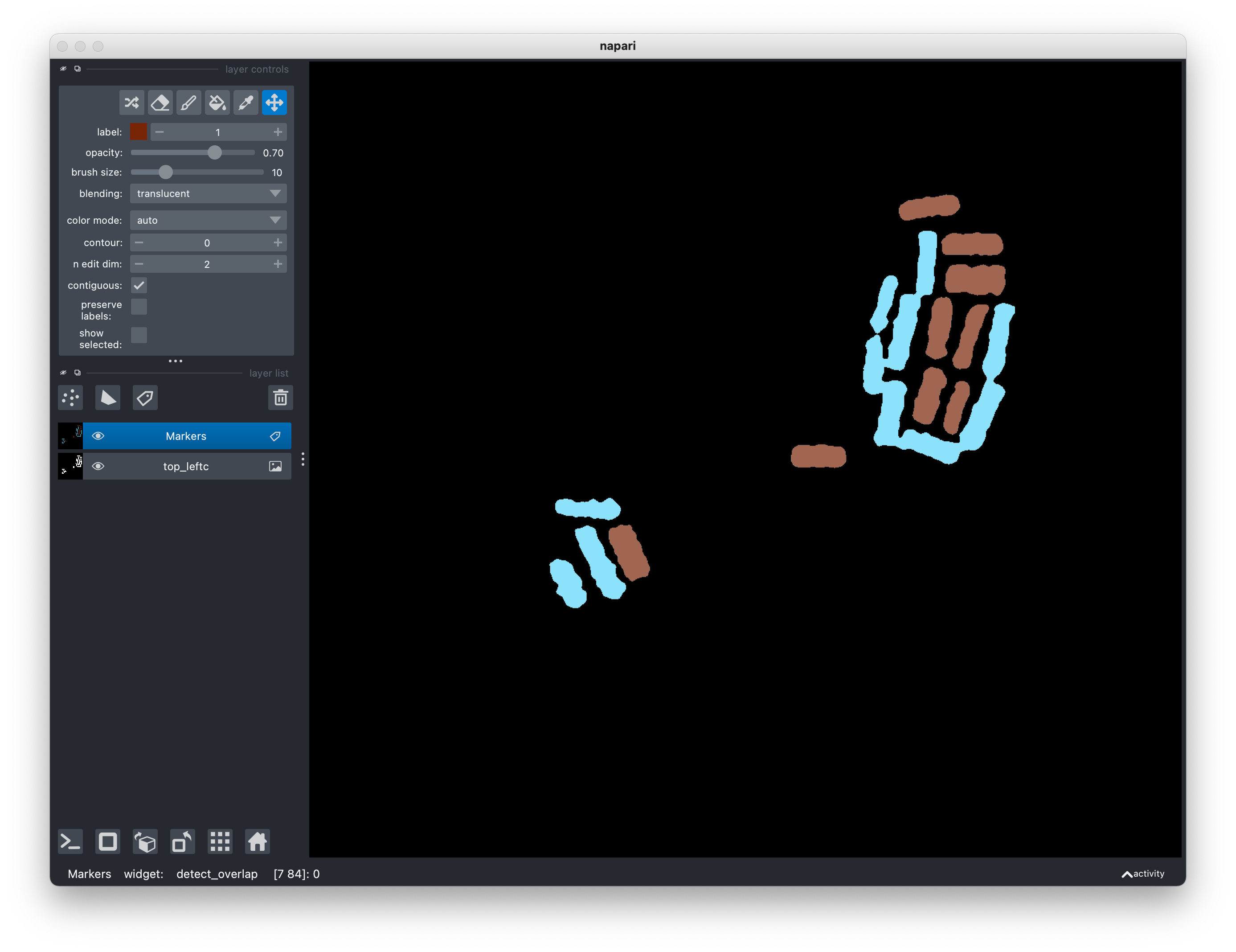
Rectangular regions are identified using oriented bounding boxes (OBB) based on tolerances for area and perimeter. All regions whose OBBs satisfy both tolerances will be considered as a rectangular object. In other words, the area_region/area_OBB <= area_tolerance and perimeter_region/perimeter_OBB <= perimeter_tolerance. The result will be a Labels layer containing at most two labels -- 1 and 2. Those with label 1 are considered as isolated rectangular regions and those with 2 are regions that are not and may need further attention.

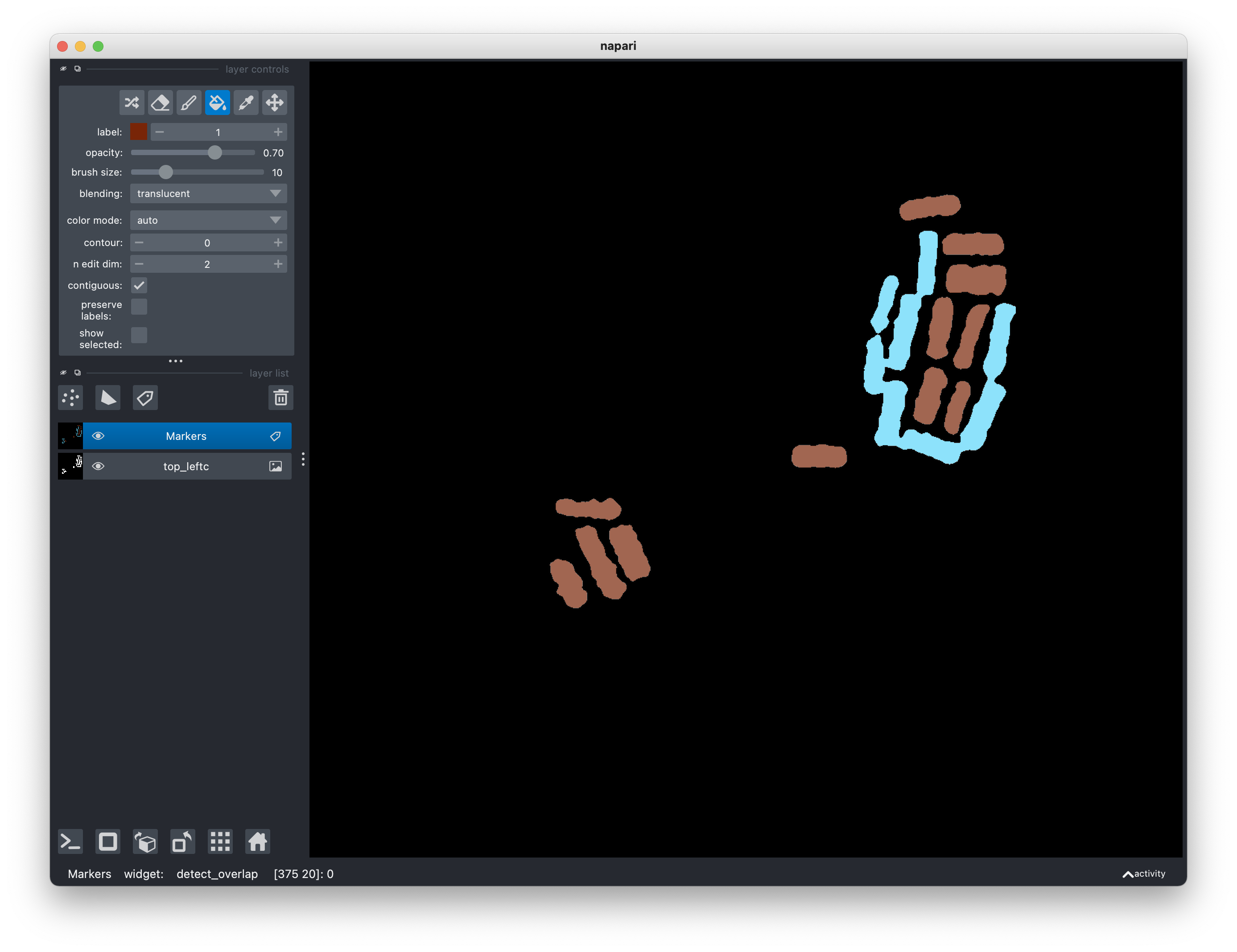
It is possible that some regions are misclassified (depends on the tolerance); use the Pick mode and Activate the fill bucket tools in the layer control panel of the viewer to assign correct labels to all regions.

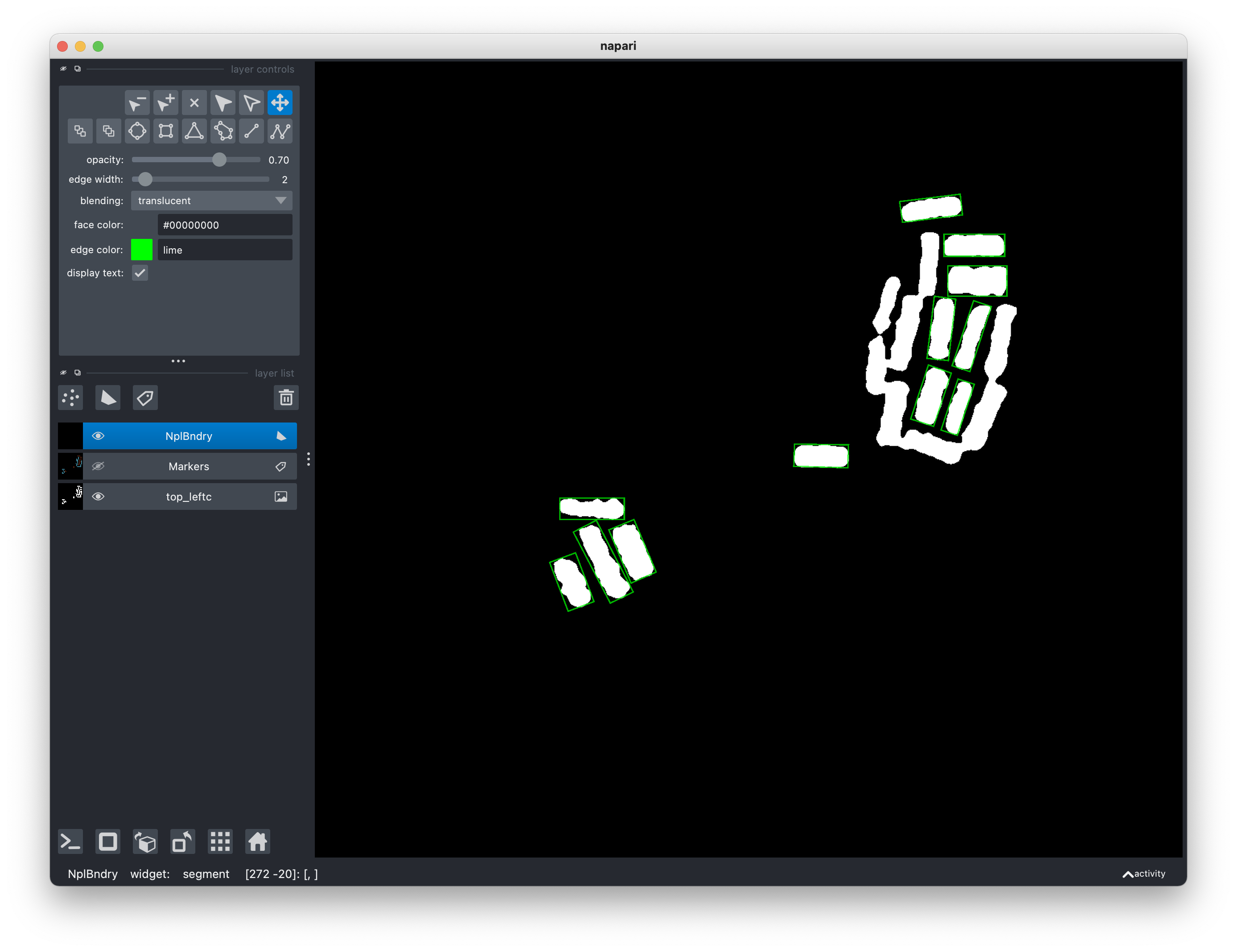
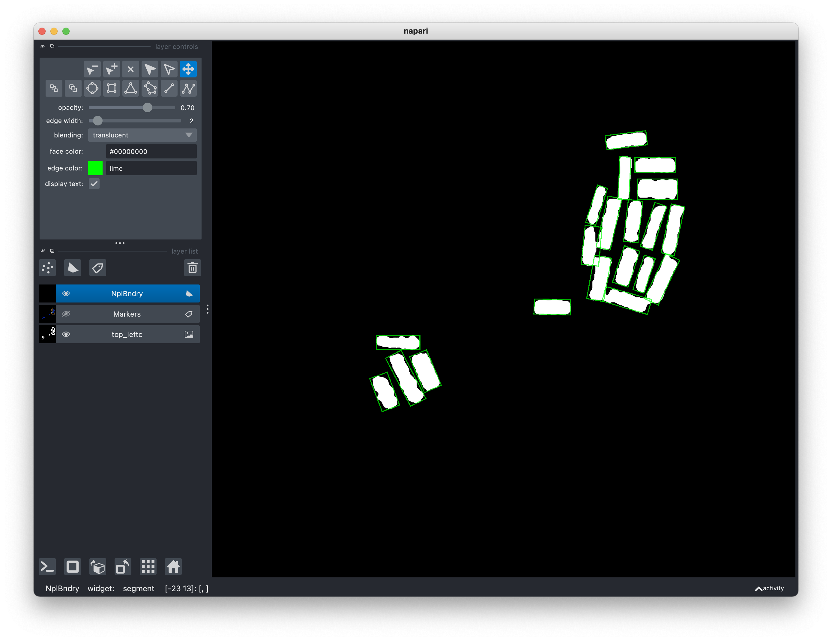
At this stage, hopefuly, most regions are classified as isolated rectangles, with a few that are not isolated. The latter may be touching rectangles or regions that are not of interest. Touching regions can be segmented with a marker-controlled Watershed algorithm. However, if you are not interested in these regions any more, just click on Window > Segmentation > Segment and bounding rectangles will appear on the regions labeled as 1.

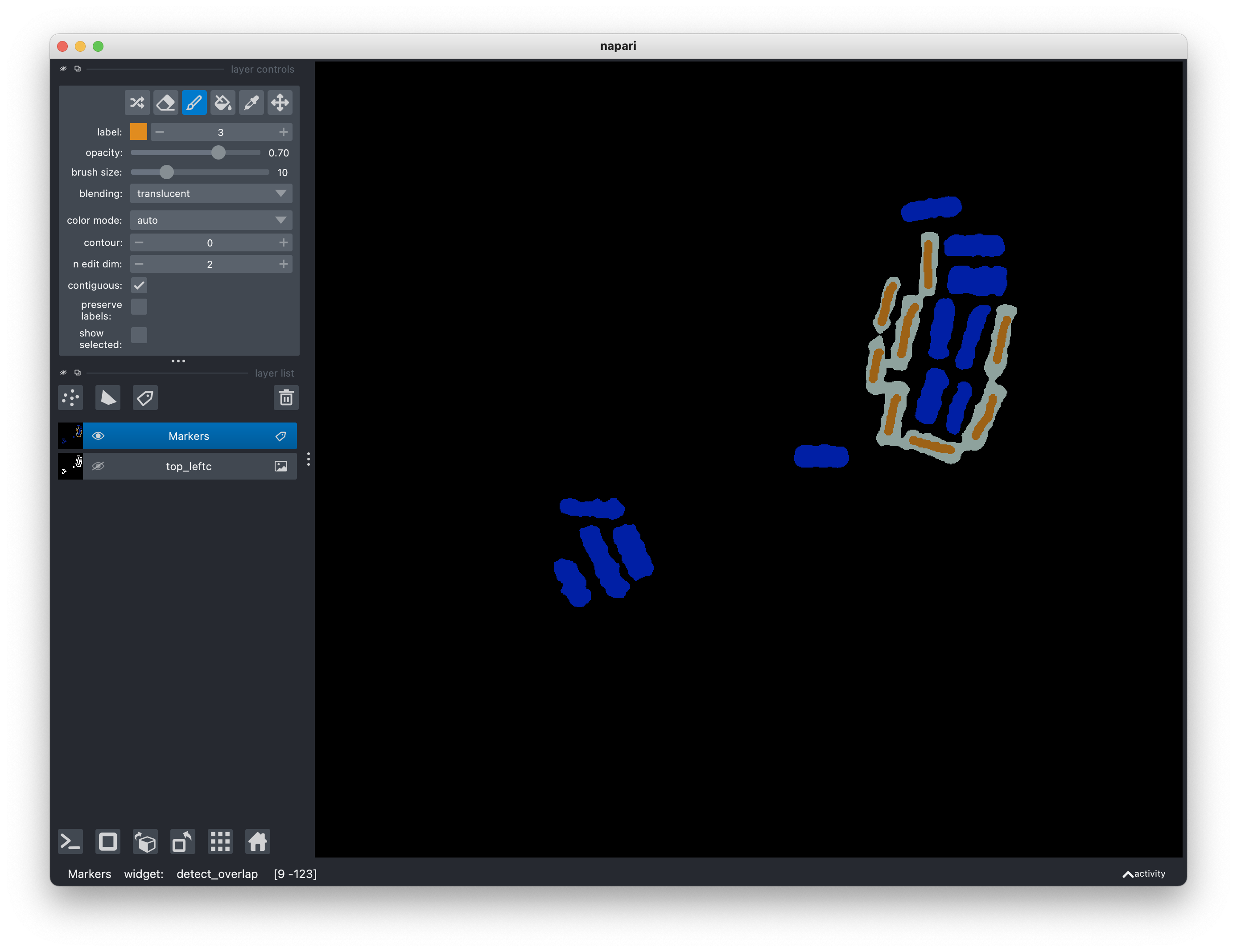
To proceed with the Watershed algorithm, use Activate the paint brush tool in the layer control panel to add markers with label 3. The number of markers should be equal to the number of segmented regions. Each marker can be a short line or even a small region, though the quality of the segmentation will greatly improve if your markers are commensurate with the desired rectangular regions. Make sure that the markers do not extend outside any region, i.e., limited within the white areas. Furthermore, if there are areas you do not wish to segment of take into further consideration, use the Activate the fill bucket tool in the layer control panel to label them as 4 or anything > 3.

Click on Window > Segmentation > Segment. In the segmentation step, you can also choose the width of the OBB edges and their color. A color is specified as a string wiht hex value (in lower case) starting with # or any of VisPy colors.

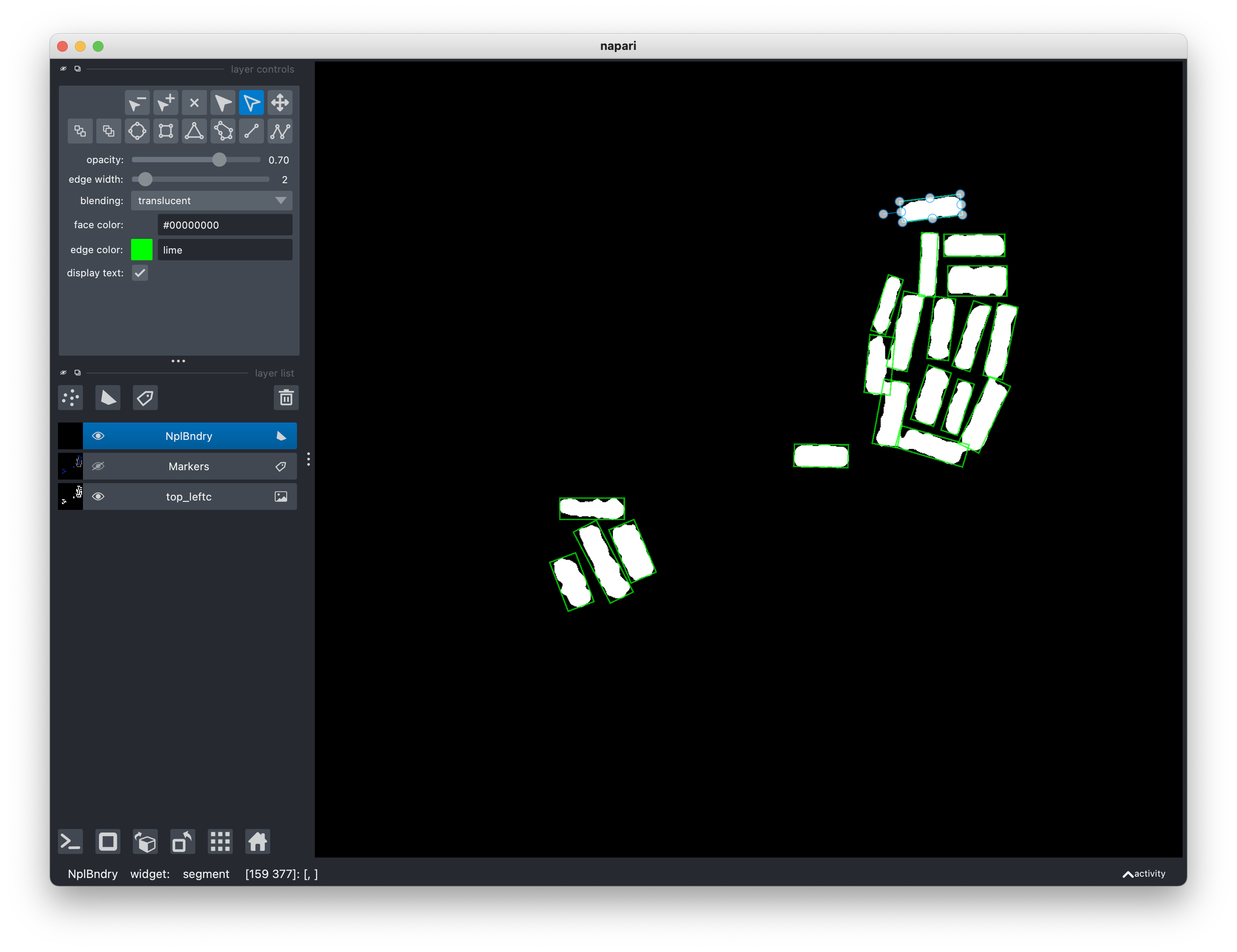
If you would like to alter the rectangles by a small amount, you can do so by directly exposing the handles on each rectangle.

In the rather unfortunate case that your original image quality is so poor that any of the preceeding steps cannot be reliably performed, you can directly add a Shapes layer and draw a bunch of rectangles.

Calculating the OBB sizes

Size statistics can be written to a file simply from Window > Get particle size. In case of input .dm3 files, the final size will be in the same unit as in the original input image. Of course, for other file formats, the sizes will be in pixels.

saridut / NPLsizer