Note: You can do whatever you want with the csv files generated in this project, no licencing involved.
This repository is for data collection and analysis of smart-devices(smartphones, tablets, watches).
The data are scraped from https://www.gsmarena.com. As of the current time, it involves 15 features namely:
- Product Name
- LTE or not (binary)
- Year announced
- Weight (in grams)
- Display type (three types: LCD, OLED, OTHER)
- Display size
- PPI (Pixels Per Inch)
- CPU (in GHz)
- Internal memory (in GB)
- RAM (in GB)
- Rear Camera (in MP)
- Front Camera (in MP)
- Bluetooth Version
- Battery (in mAh)
- Price (in USD)*
- Some prices listed on the website were in foreign currencies, the appropriate current exchange rate has been applied to convert the prices to USD (as of 12/30/2018)
Currently, I am aiming at about 2000 devices (inclusive of smartphones, tablets and watches), from about 40 manufacturers.
- Generate a well documented dataset summarising the above mentioned features for over 2000 devices.
- Employ various supervised regression techniques like linear, natural splines, including tree-based methods like random-forests.
- Use this as an educational dataset to experiment with validation techniques like cross-validation and bootstrap.
- Explore patterns in the data by employing unsupervised techniques like PCA and Clustering.
So far, I have achieved to scrap,clean and compile into csv, data for more than 1000 phones/tablets/watches. Attaching a screenshot of the clean csv :

============================================================
Note: For all the plots below, the R code and the console output of RStudio can be found in the R_dump_xx.dat files.
Here I try to employ PCA on 9 features:
- Weight (in grams)
- screen_size (inches)
- PPI
- cpu_ghz (in GHz)
- RAM (in GB)
- Internal memory (in GB)
- Camera (in MP)
- Battery (in mAh)
- Price (in USD)
The other features are ommitted because either they are non-numeric or have less than 5 non-unique values in total. The PCA spit out 9 components, but as expected, the first two components explain more than 50% varaince. The loadings of each feature and the variance explained by each principal component can be inferred from the following R output:
> data=read.csv('~/Desktop/Experiments/Smartphone Price/csv/data_clean.csv')
> names(data)
[1] "name" "LTE" "year" "weight" "display_type"
[6] "screen_size" "ppi" "cpu_ghz" "ram" "internal"
[11] "camera" "front_cam" "blth_v" "battery" "price"
> keeps = c('weight','screen_size','ppi','cpu_ghz','ram','internal','camera','battery','price')
> data = data[keeps]
> names(data)
[1] "weight" "screen_size" "ppi" "cpu_ghz" "ram"
[6] "internal" "camera" "battery" "price"
> pca.out = prcomp(data,scale=TRUE)
> pca.out
Standard deviations (1, .., p=9):
[1] 2.1676360 1.4247753 0.9333816 0.6446664 0.5695935 0.4640132 0.4580829 0.3773277
[9] 0.3043232
Rotation (n x k) = (9 x 9):
PC1 PC2 PC3 PC4 PC5 PC6
weight -0.1702557 -0.61499648 0.11466072 -0.24107137 0.06229698 -0.05427148
screen_size -0.3208003 -0.44646115 -0.16795676 0.12601336 0.02399054 -0.34171744
ppi -0.3341030 0.33014336 -0.25691627 -0.37983090 0.40853834 0.36601715
cpu_ghz -0.4106557 0.09871307 -0.13658769 0.16226295 0.44487316 -0.51814113
ram -0.3972893 0.18558905 -0.02842717 0.38947693 0.12565417 0.26251748
internal -0.3416498 0.08711022 0.55041231 0.48023737 -0.23346237 0.13150173
camera -0.3312704 0.26695962 -0.39805456 -0.16988601 -0.72963617 -0.24050782
battery -0.3209574 -0.41828210 -0.19463396 -0.05087644 -0.16151820 0.56313403
price -0.3170490 0.12431418 0.61146517 -0.58449515 -0.04446480 -0.12912372
PC7 PC8 PC9
weight -0.05815725 0.45834294 0.548856112
screen_size -0.19730973 0.14724298 -0.689719337
ppi -0.48343876 0.17709677 -0.056165921
cpu_ghz 0.08299903 -0.42759152 0.347169198
ram 0.59216310 0.46589439 -0.052899872
internal -0.50416293 -0.05104836 0.116284010
camera -0.02232512 0.10895156 0.170592994
battery 0.16416756 -0.55797963 0.007439038
price 0.29120086 -0.10567993 -0.232132429
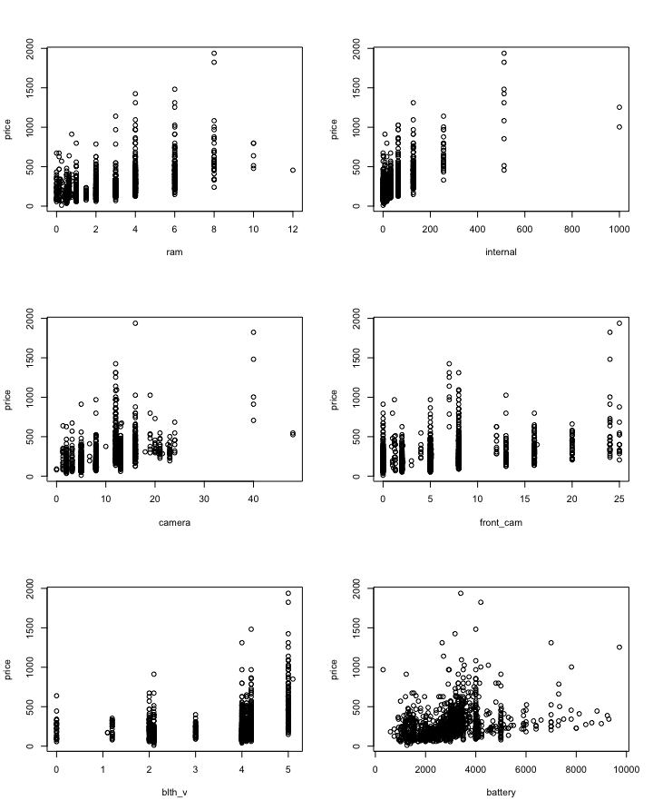
Below are the plots of price vs each column. Visually we can determine columns which take up most and least amount of variance in the data.
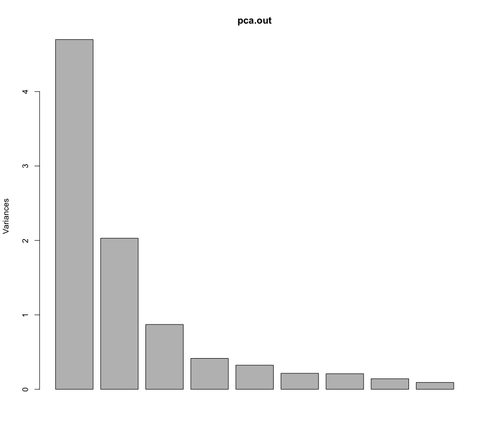
Hence, only the first two components carry most of the variance. In the R output above, the loadings of each feature for each components can be seen, but its not very intuitive. Thanks to R, we can plot the loadings of all the features in a single plot.
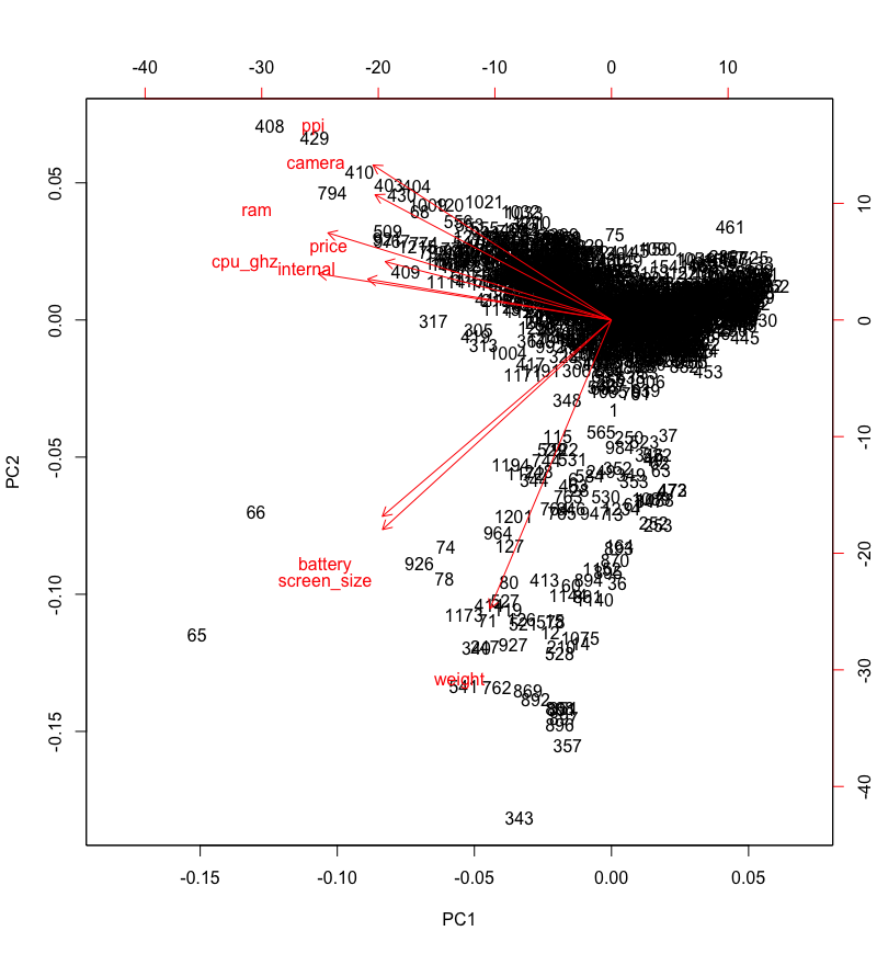
We can see that none of the features get very close to the components, which was expected. Because if that were true, then a single feature would carry most of the variance. As far as mobile phones/tablets are concerned, that can hardly be the case.
Its notable though that internal,ram,cpu_ghz and price get the closest to the first principal component, which means that mobile phones/tablets vary in these features the most as compared to the other 7 features.
Meanwhile, weight is the closest to the second principal component, which means that weight varies quite a bit too, but that's no surprise.
=============================================================
Below is a plot of price vs each feature in the entire data.

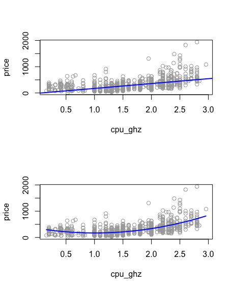
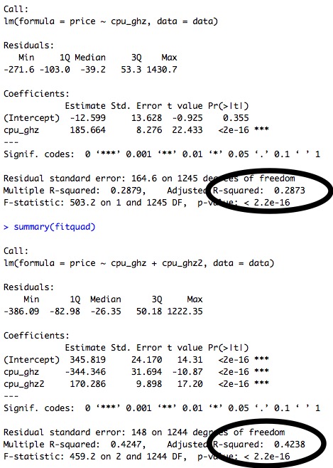
Adjusted R-squared values indicate that the linear model explains about 29% of the total variance, whereas the quadratic model explains 43% of the total variance, as below:
require(gam)

gam1 = gam(price~s(cpu_ghz,df=4)+s(ppi,df=4)+s(screen_size,df=4),data=data)
summary(gam1)
Call: gam(formula = price ~ s(cpu_ghz, df = 4) + s(ppi, df = 4) + s(screen_size,
    df = 4), data = data)
Deviance Residuals:
    Min      1Q  Median      3Q     Max
-337.16  -75.08  -23.70   49.56 1264.79

(Dispersion Parameter for gaussian family taken to be 18835.41)

    Null Deviance: 47336465 on 1246 degrees of freedom
Residual Deviance: 23242893 on 1234 degrees of freedom
AIC: 15828.6
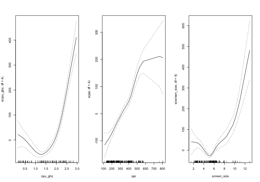
Using only three, and highly noisy features results in a pathetic fit with high error bars, especially towards the endpoints. The resulting fit had an atrociously high AIC index of 15828.6 (refer R_dump_1.dat). But we can visualise the trend of the dependence of each of the three variables, through the plots below:
Here I train a random forest over all 13 features of the data. Using 4 features at each split of the tree, we get a 70.65% explanation of the total varaiance, which is not bad! (refer R_dump_randomForest.dat for detailed console output)
> data=read.csv('data_clean.csv')
> attach(data)
> require(randomForest)
> train = sample(1:nrow(data),900)
> rf.data = randomForest(price~.-name-price_category,data=data,subset=train)
> oob.err=double(13)
> test.err=double(13)

> rf.data

Call:
 randomForest(formula = price ~ . - name - price_category, data = data)
               Type of random forest: regression
                     Number of trees: 500
No. of variables tried at each split: 4

          Mean of squared residuals: 11141.51
                    % Var explained: 70.65
In a different approach, the data set is divided into a training set (900 entries) and a test set (300 entries). To have a better judgement of how many features to consider at each split, the Out of bag error and Test error are plotted for different value of features:
> for(mtry in 1:13){
+     fit=randomForest(price~.-name-price_category,data=data,subset=train,mtry=mtry,ntree=500)
+     oob.err[mtry] = fit$mse[500]
+     pred=predict(fit,data[-train,])
+     test.err[mtry]=with(data[-train,],mean((price-pred)^2))
+     cat(mtry," ")
+ }
1  2  3  4  5  6  7  8  9  10  11  12  13
> matplot(1:mtry,cbind(test.err,oob.err),pch=19,col=c('red','blue'),type='b',ylab='Mean Squared Error',xlab='# of features at each split')
> legend("topright",legend=c("Out of bag","Test"),pch=19,col=c("red","blue"))
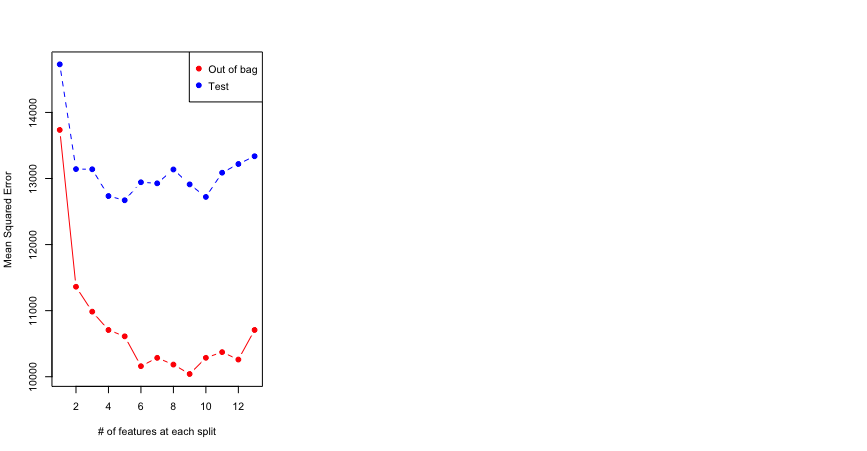
Looks like in this case the OOB error does not do a decent job in predicting the test error. Also, there is not a lot of change in the test error for anything between 4 and 8 features at each split. Hence I keep it at 4 (simpler the better).
For the purpose of classification. I divided the devices into three classes:
- Cheap devices: costing $200 or less
- Not-so-cheap devices: costing between $200 - $500
- Expensive devices: costing $500 and above
> require(MASS)
Loading required package: MASS
> fitlda = lda(price_category~.-name-price,data=data,subset=train)
> fitlda
Call:
lda(price_category ~ . - name - price, data = data, subset = train)

Prior probabilities of groups:
         1          2          3
0.42444444 0.47777778 0.09777778

Group means:
        LTE     year   weight display_typeOLED display_typeOTHER screen_size      ppi  cpu_ghz      ram  internal    camera front_cam
1 0.6596859 2015.508 155.2094       0.02879581        0.26963351    4.933168 264.8141 1.291107 1.674450  17.73530  8.486518  3.968325
2 0.7790698 2015.258 192.6349       0.15348837        0.18372093    5.555233 335.1279 1.617312 2.999730  46.57702 11.764767  7.553721
3 0.9318182 2016.602 205.0909       0.59090909        0.09090909    5.991136 411.5341 2.227284 5.135455 160.85255 14.868182 10.812500
    blth_v  battery
1 3.625654 2574.725
2 3.819302 3260.174
3 4.400000 3568.307

Coefficients of linear discriminants:
                            LD1           LD2
LTE                0.3051819153 -0.5573399936
year              -0.3332056905  0.4466952185
weight             0.0072860994  0.0037372107
display_typeOLED   0.8933229494  1.4194517138
display_typeOTHER  0.2626532661  0.1605923964
screen_size       -0.2039114518 -0.5398919819
ppi                0.0032347057 -0.0039307720
cpu_ghz            0.9791124094  0.2700175880
ram                0.1553809657 -0.0438809386
internal           0.0043088153  0.0106483916
camera             0.0358542407 -0.0183217878
front_cam          0.0415875543 -0.0887501794
blth_v             0.1240752051 -0.0717548012
battery           -0.0000060288 -0.0003019114

Proportion of trace:
   LD1    LD2
0.8325 0.1675
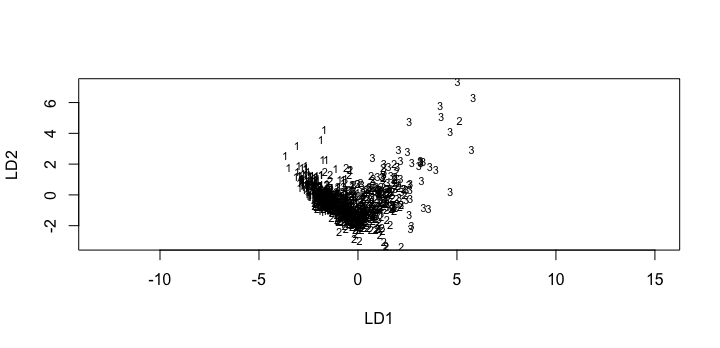
The aim here is to use LDA to classify devices into their respective categories. After employing LDA for the three classes (labelled as 1,2,3), the classification along each of the Linear Discriminants can be plotted as a graph : (three classes so 2 discriminants):
We can also see the confusion matrix, which gives us a better understanding of how well the model performed:
  1   2   3
1 103  40   1
2  34 121  12
3   0  16  20
The confusion matrix is tending towards being diagonal, which means the model preformed pretty well. We can also see the mean rate of correct classification, which can be a measure of the test accuracy.
> mean(lda.pred$class==data[-train,]$price_category)
[1] 0.70317
70.31% times, the model correctly classified the devices, which is pretty good for such a dumb model!