Reinforcement learning for quantum state preparation
Author: Sarang Zambare
This repository is a part of a project I undertook at the Indian Institute of Technology, Bombay. I demonstrate a basic way in which reinforcement learning can be used to prepare a given quantum state, from a given initial state.
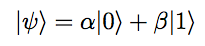
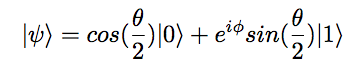
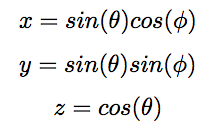
In this particular demonstration, I keep things simple and assume that the quantum state in question is a two level system, and an arbitrary state can be represented as :
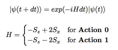
To transform the state from one to the other, I use the bang-bang protocol, also known as hysteresis control or 2-state control in control theory, to switch between two hamiltonians being operated to the quantum state at each time instant. The two hamiltonians I used are the ground state hamiltonians given by:
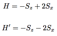
The control parameter that I use is the magnetic field, which can be +2 or -2 (this is also the coefficient of Sx in the hamiltonians)
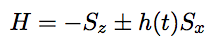
where h(t) is the magnetic field and the control parameter.
Q-learning algorithm :
Reinforcement learning is an area of machine learning inspired by behaviourist psychology, concerned with how software agents ought to take actions in an environment so as to maximize some notion of cumulative reward. The problem, due to its generality, is studied in many other disciplines, such as game theory, control theory, operations research etc. A specific type of reinforcement learning is the Watkins Q-learning algorithm. Q-learning algorithm has the following constituents:
- Agent: An agent can be thought of as an imaginary being, taking all the actions and experi- encing rewards in the process. Depending on the formulation of the problem, an agent’s aim is to minimise or maximise its reward, and in doing so, take the optimal course of actions.
- State: Any Q-learning problem should have a starting state and a terminal state, along with a number of intermediate states. Any action taken by the agent can change the state of the system. States can be thought of as stepping stones that the agent has to walk through to get to the final state from the initial state.
- Action: Corresponding to each state, there is a set of possible actions that the agent can take. The agent’s aim is to select the right action at each state so as to optimise reward.
- Reward: Corresponding to each state and action pair, a reward is associated.
- Q function: Each state and action pair has a Q(s, a) associated. The Q-value can be interpreted as the selectibility of a particular action at a given state. Actions with higher Q-value are favoured over actions with lower Q-value. The Q function is given by
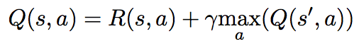
where • s is the state • a is the action • R(s, a) is the reward function • s' is the next state, i.e. the state resulting from taking action a at state s
Formulation of the problem :
The problem of finding the right choice of h(t) so as to prepare the target state, has to be modelled in a way that is compatible with the Q-learning requirements. Therefore, we need to define states, actions, rewards and the Q-matrix. Suppose we have to prepare the state in time T, and our smallest time step is dt, then for every time step dt, we have the option of keeping the magnetic field as +2 or 2. Therefore, we define a state by the couple
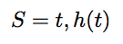
Where S denotes the set of states.
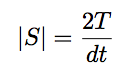
For every possible time t , we have two possible values of the magnetic field, therefore the number of states is :
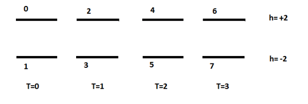
For example, lets say T = 4 and dt = 1, then the states would be depicted as follows:
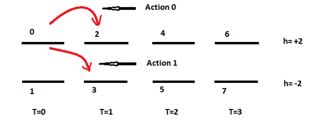
For every state, there are two possible actions, lets call these as Action 0 and Action 1, and they are depicted as follows:
Every reinforcement learning agent needs a measure of reward which is tries to maximise. In this problem, reward is determined by how close the agent is able to prepare the final state to the intended state. Accordingly, the reward function is determined as :
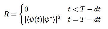
In the above steps, we calculate the state at time (t+dt) by applying the time evolution operator to the state at time t :
When this algorithm is implemented, after many episodes, the Q-matrix thus formed will contain the right choices of magnetic field values at each time step. Keep in mind that the above algorithm is for constructing the Q-matrix only. To discern the optimal choices of fields at every time step, we select the action which has a higher Q-value of the two. If the Q-values are same for the two actions, then it doesn’t matter which action we take, and hence we choose randomly from the two actions.
Results:
After calculating the value of the magnetic field at every time step, we finally calculate the fidelity of the prepared quantum state :
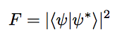
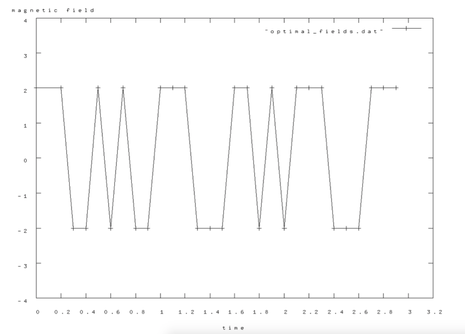
The Q-learning algorithm mentioned above was implemented using Python. The total ramp time was set to be T = 3 and each time step was dt = 0.1. The learning rate was set to 0.2 and the initial and target quantum states used were the same as mentioned in the previous sections of this report. The values of magnetic field that we used for the bang-bang protocol were ±2. I ran the algorithm for a total of 10,000 episodes, and the maximum fidelity I achieved was 99.5%
Any quantum state of a two level system can be represented as a 3D vector on the bloch sphere, where the state can be decomposed as:
and the bloch vector is given by the following components:
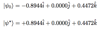
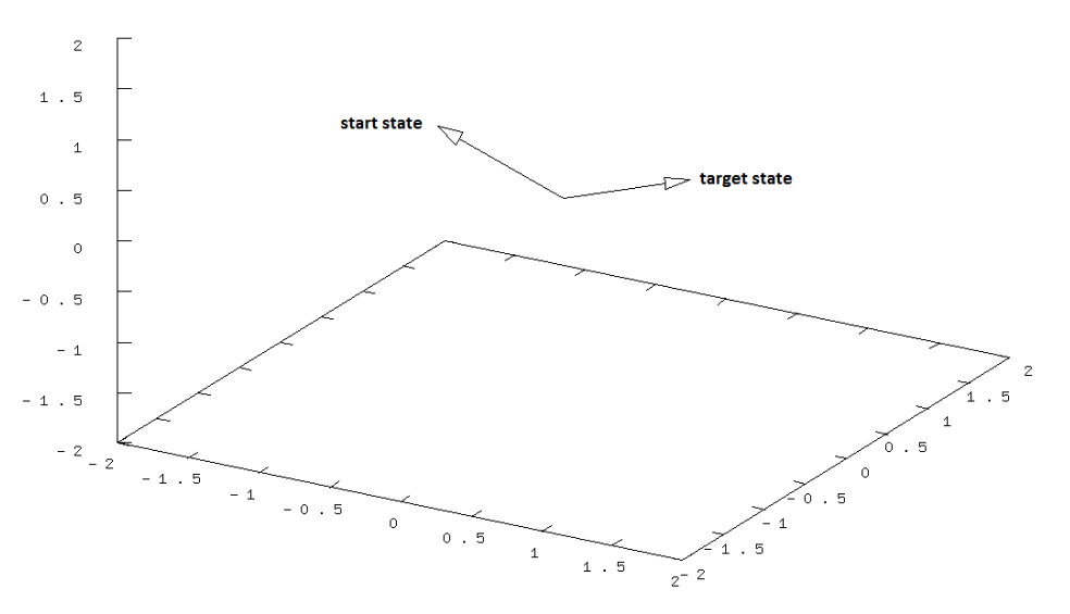
In this particular example, the start and final state I used can be decomposed as :
After plotting them on the bloch sphere, they look like so :
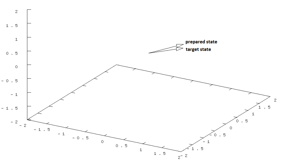
After being subjected to the driving protocol that the Q-learning algorithm learned, the maximum fidelity I got was 99.5%. The final prepared state looks like so:
The optimal values of magnetic field at each time step is illustrated in the following figure:
An animated video of the agent learning to move towards the given final state can be found in the vid folder of the repository. It shows the agent's steps when its trained only for 100 episodes, vs when it is trained for 10,000 episodes.