sanjay035 / StochasticGradientDescent

Customized implementation of Stochastic Gradient Descent for Linear Regression that optimizes the weights "W(i)" of each components and the bias "b" term.

StochasticGradientDescent

A custom implementation of Stochastic Gradient Descent for Linear Regression that optimizes the weights W(i) of each component and the bias b term.

Gradient Descent:

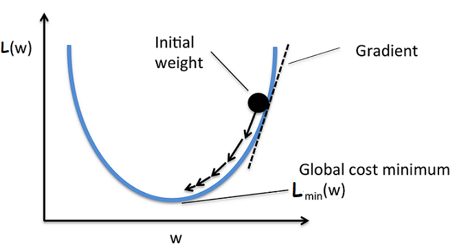
Gradient Descent is an iterative optimization algorithm that can be used to converge to an optimal value easily with the use of modern computaional power.

• The update equation for every iteration is, x(i) = x(i-1) - r * [df/dx]_x(i-1) ; i : 1 -> n.
• It mainly depends on the learning rate (or) step size denoted by "r".
• The learning rate tells how fast to converge to the optimal value. So giving a right value of "r" matters.
• If the right value of "r" ain't given then the updation might jump over optimal value(min) and we'll not be converging at the right solution. Hence need to check with different values of "r".

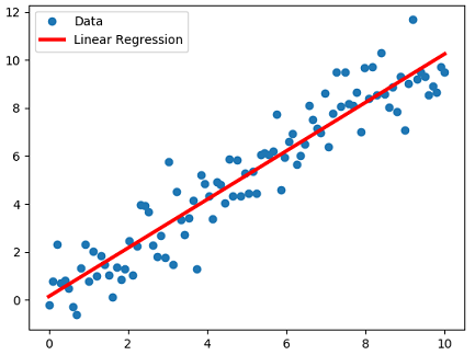
Let us consider a simple linear regression,

• Objective : Find the line/plane that best fits the data as,

• The dataset is D = <x_i, y_i> ; x_i ∈ R^d ; y_i ∈ R. Here d is for # of dimensions.
• We can find the line/plane that fits the real values data of form y_i = W.T*x_i + B for given x_i. Here B is for bias.
• Then we've Mean Squared Error(MSE) = sum( [y_i - (W.T*x_i + B)]^2 ) / n ; i : 1 -> n.
• The optimal weight vector will be W* = argmin(W) sum( [y_i - (W.T*x_i + B)]^2 ) / n i.e the one which gives minimum sum of squared errors.

We can write the optimization problem W* = argmin(W) sum( [y_i - (W.T*x_i + B)]^2 ) / n as,

L(W) = [ 𝜮(y_i - (W.T*x_i + B))^2 ] / n ; i : 1 -> n.

Then the vector differentiation or grad of L(w) is 𝞩_w L = 𝜮 { 2*(y_i - (W.T*x_i + B))(-x_i) } / n

Steps for finding Optimal weight:

1. Initialize the weight vector W(0) with random values.
2. repeat until W(k-1) and W(k) doesn't change much:
   • W(i) = W(i-1) - r*𝜮 { (-2*x_i)*(y_i - (W(i-1)*x_i + B)) } / n ; i : 1 -> n
3. Declare W* = W(k-1)
4. Similarly step 2 & 3 can be followed to get the optimal value of bias "B" term where instead of differentiating with respect to W we do it with B.

But the problem with gradient descent is it takes a lot of time calculating 𝜮 { (-2*x_i)*(y_i - (W.T*x_i + B)) } / n for every iteration as i : 1 -> n.

To overcome this we can select K random points instead of total n points at each iteration for the above summation.

This technique of selecting K random points at each iteration is known as Stochastic Gradient Descent. Stochastic here is for randomization.

• So here the updation looks like, SGD : W(i) = W(i-1) - r*𝜮 { (-2*x_i)*(y_i - (W(i-1)*x_i + B)) } / K with i: 1 -> K

It also can be seen that W* of GradientDescent is almost equal to W* of Stochastic Gradient descent but with some increased number of iterations in Stochastic Gradient descent for the convergence of optimal value.

__ K is often called as batch size in Stochastic Gradient descent(SGD).

• If K=1 then it's simple SGD.
• If 1<K<<n then it's batch SGD with batch size = K.

Hence, Stochastic Gradient descent(SGD) is one of the most important optimization algorithm in Machine Learning.

Note:

Again gradient descent can stuck in local optima if the function to be optimized is a non-convex.

In the above exmaple of linear regression we were able to find the optimal value without being stuck at local optima as the sum of squared errors is a convex function.