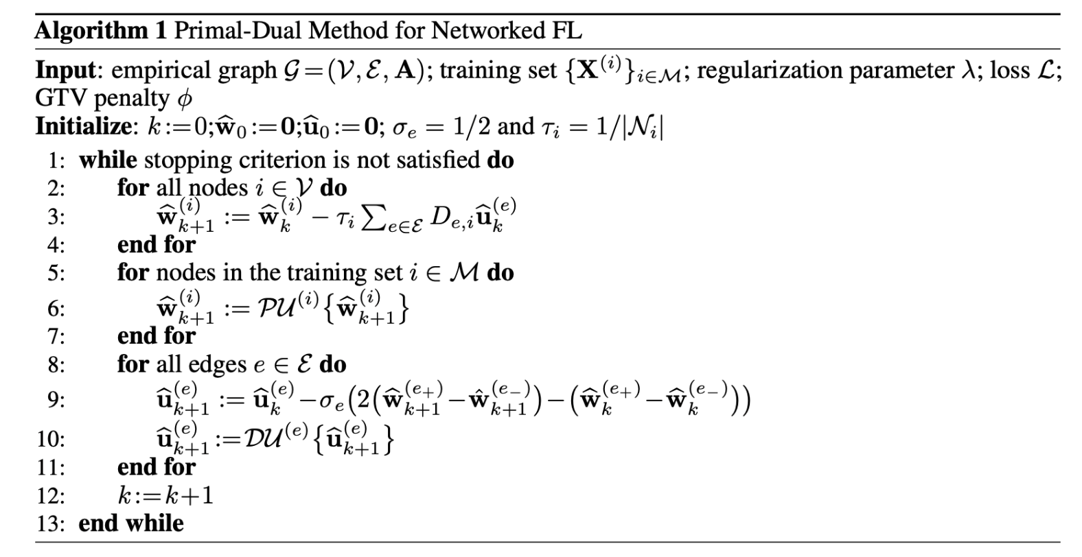
This repository is the official implementation of Networked Federated Multi-Task Learning paper.
The package related to the algorithm implementation is algorithm which has the following structure.
- main.py
- the implementation of algorithm 1
- optimizer.py
- the primal optimizer for the loss functions, we have implemented
the squared error loss, and the logistic loss with
pytorchand also the straight forward primal optimizer in the Networked Linear Regression section which is much faster than thepytorchone
- the primal optimizer for the loss functions, we have implemented
the squared error loss, and the logistic loss with
- penalty.py
- the different penalty functions for the dual optimizers explained in the paper,
norm2,MOCHA, andnorm1
- the different penalty functions for the dual optimizers explained in the paper,
For running your own primal and dual optimizers you can inherit a class from class Optimizer
and class Penalty respectively.
This Algorithm does not need any computational resource type and all the experiments have run on my own laptop which is a standard macbook (Quad-Core Intel Core i5 and 8 GB RAM), just the bottleneck might be RAM, if you have a dataset such that its network has a large number of nodes/edges, you might need to run the algorithm in a system with the required RAM.
To install requirements:
pip install -r requirements.txt
📋 For running the code you need to have python 3.7
In this repository we have multiple experiments
As mentioned in the paper, Algorithm 1 will predict almost the same weight vectors for the nodes within the well-connected clusters. So one reasonable experiment would be a network with stochastic block structure.
- With Two Clusters: This SBM has two clusters |C1| = |C2| = 100.
Two nodes within the same cluster are connected by an edge with probability
pin=0.5, and two nodes from different clusters are connected by an edge with probabilitypout=0.01. Each node i ∈ V represents a local dataset consisting ofmfeature vectors x(i,1), ... , x(i,m) ∈ Rn . The feature vectors are i.i.d. realizations of a standard Gaussian random vector x ~ N(0,I). The labels yi1, ... , yim ∈ R for each node i ∈ V are generated according to the linear model yir = (x(i, r))Tw̄(i) + ε , with ε ∈ N(0,σ), weight vector w(i) = (2, 2)T for i ∈ C1, and w(i) = (-2, 2)T for i ∈ C2. The tuning parameter λ in algorithm1 is manually chosen, guided by the resulting MSE, as λ = 0.01 for norm1 and norm2 and also λ = 0.05 for mocha penalty function. We assume that labels y(i) are available for 40% of the graph nodes. We randomly choose the training set M and use the rest as test set. As the result we compare the mean MSE of Algorithm 1 with plain linear regression and decision tree regression with respect to the different random sampling sets, please see the implementation at SBM_experiment.ipynb.
| Method name | Train MSE | Test MSE |
|---|---|---|
| algorithm 1, norm1 | 9.78e-06 | 1.06e-05 |
| algorithm 1, norm2 | 9.80e-06 | 1.06e-05 |
| algorithm 1, mocha | 0.0012 | 0.0633 |
| plain linear regression | 3.720 | 4.031 |
| decision tree regression | 3.762 | 4.499 |
- With Five Clusters: The size of the clusters are {70, 10, 50, 100, 150} with random weight vectors ∈ R2 selected uniformly from [0,1) . We run Algorithm 1 with a fixed pin = 0.5 and pout = 0.001, and a fixed number of 1000 iterations. The tuning parameter λ in algorithm1 is manually chosen, guided by the resulting MSE, as λ = 0.01 for norm1 and norm2 and also λ = 0.05 for mocha penalty function. We assume that labels y(i) are available for 20% of the graph nodes. We randomly choose the training set M and use the rest as test set. As the result we compare the mean MSE of Algorithm 1 with plain linear regression and decision tree regression with respect to the different random sampling sets, please see the implementation at SBM_experiment.ipynb.
| Method name | Train MSE | Test MSE |
|---|---|---|
| algorithm 1, norm1 | 3.83e-06 | 7.93e-06 |
| algorithm 1, norm2 | 4.24e-06 | 5.72e-06 |
| algorithm 1, mocha | 9.15e-06 | 0.0012 |
| plain linear regression | 0.1383 | 0.1485 |
| decision tree regression | 0.2973 | 0.3483 |
This dataset is constructed by adding elevation information to the 3D road network in North Jutland, Denmark (covering a region of 185 × 135 km2), containing LATITUDE, LONGITUDE, and also ALTITUDE of regions. We consider a graph G represents this dataset, which its nodes are the regions of the dataset and are connected by edges to their nearby neighbours with the weights that are related to the distances between them. So the feature vector X(i) ∈ R1*2 of node i ∈ V contains the latitude and longitude of its corresponding region, and the label y(i) ∈ R is its altitudes.
We use Algorithm 1 to learn the weight vectors w(i) for a localized linear model. We assume that labels y(i) are available for 30% of the graph nodes, thus, for 70% of the nodes in G we do not know the labels y(i) but predict them with the weight vectors ŵ(i) obtained from Algorithm 1 (using a fixed number of 1000 iterations, and λ = 0.2). We randomly choose the training set M and use the rest as test set. As the result we compare the mean MSE of Algorithm 1 with plain linear regression and decision tree regression with respect to the different random sampling sets, please see the implementation at 3d_road_experiment.ipynb.
| Method name | Train MSE | Test MSE |
|---|---|---|
| algorithm 1, norm1 | 0.0243 | 24.625 |
| algorithm 1, norm2 | 0.0236 | 24.621 |
| algorithm 1, mocha | 2.03e-05 | 20.977 |
| plain linear regression | 286.44 | 289.65 |
| decision tree regression | 167.42 | 175.36 |
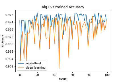
In this section, we tested our method with Tensorflow ”cats vs dogs” Classification Dataset. Each node of the empirical graph G stands for a deep neural network in which the base model is Xception (with 132 layers) and has trained on the ImageNet dataset, also the new model containes a Global Average Pooling 2D, a Dropout, and a Dense layer (with linear activation, Adam optimizer, and Binary Cross Entropy loss function) respectively. The difference between the nodes is their training datasets. Suppose that the training dataset for the node i is img1, ..., imgt, we consider the result of the base model for the rth train image (imgr) as the feature vector (x(i, r)), and the result of the new model as its label (yir), and wi is the weight vector of its Dense layer and the aim of this experiment is to estimate the weight vectors, wi of all the nodes.
The total number of nodes is 100, each node is connected to its 3 nearest neighbours, the ones with the highest weights. We select 20 random nodes as the samplingset for Algorithm 1 (with λ = 0.001 and a fixed number of 1000 iterations). Our method has increased the overall accuracy of the nodes in a significant shorter time, the needed time for training each model with three learning epochs is almost 20 minutes, so training 100 models lasts 2000 minutes, while the computation time for our algorithm itself is less than 5 minutes. by adding the time for training the sampling set, which is 20 nodes, the total time would be 405 minutes (405 << 2000).
Fig: The accuracy for each model obtained after 1000 number of iterations used in Algorithm 1 based on the squared error loss . In this figure, the blue line shows the accuracy of the models based on the weights estimated by our method and the orange line shows the accuracy of the models by training its weights by the deep neural network after three epochs.
See the implementation at deep_learning_experiment.ipynb. (Just note that loading the trained deep learning data and creating the corresponding graph is rather time consuming.)
This repository is distributed under the BSD 3-Clause License.

