#Running on S3DF
In case you are running all over from scratch the hits2h5, this is likely a good script-ish thing to do:
Be sure the create the 'h5files' in the scratch subdirectory.
source /sdf/group/lcls/ds/ana/sw/conda3/manage/bin/psconda.sh
export scratchpath=/sdf/data/lcls/ds/tmo/tmox42619/scratch/ryan_output_debug/h5files
export datapath=/sdf/data/lcls/ds/tmo/tmox42619/xtc
export expname=tmox42619
export nshots=100
export configfile=${scratchpath}/${expname}.hsdconfig.h5
python3 ./src/set_configs.py ${configfile}
python3 ./src/hits2h5.py <list of run numbers>
#Working with already pre-processed h5 fileson s3df
source /sdf/group/lcls/ds/ana/sw/conda2/manage/bin/psconda.sh
conda deactivate
conda activate h5-1.0.1
python3 ./src/batchQuantizeHits.py 16 128 /sdf/data/lcls/ds/tmo/tmox42619/scratch/ryan_output_multiretardation/h5files/hits.tmox42619.run_132.h5
e.g. that gives 16 batches each using 128 bins for the tof dimension.
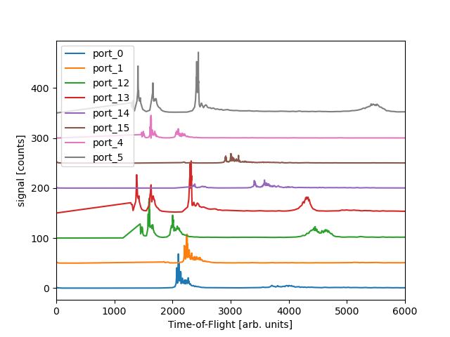 We see the different spectra for each of the ports. This is for the quantized combination of runs 131-133.
We take as the calibration points the rough position of the features along with the various expected energies given 600eV photon enerrgy.
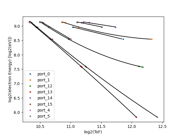
Runs 132-134, using ./src/Calib_Multiretardation.py we get the following fit values in E(i) = theta0 + theta1*i + theta2* i**2 then prints output:
coffee@pslogin03:x42619$ ./src/Calib_Multiretardation.py
port_0 fit  nam (300,400)   :   390.167 -0.168  0.000
port_0 fit  oam (400,525)   :   499.806 0.606   -0.033
port_1 fit  nam (300,400)   :   368.766 0.109   -0.001
port_1 fit  oam (400,525)   :   508.829 -0.249  -0.005
port_1 fit  IV (525,600)    :   569.103 -1.355
port_12 fit n1s (100,300)   :   212.450 -0.156
port_12 fit nam (300,400)   :   415.556 -1.297  0.008
port_12 fit oam (400,525)   :   519.394 -1.160  -0.003
port_12 fit IV (525,600)    :   564.891 -0.955
port_13 fit n1s (100,300)   :   219.296 -0.577
port_13 fit nam (300,400)   :   419.980 -3.328  0.050
port_13 fit oam (400,525)   :   528.780 -6.415  0.247
port_13 fit IV (525,600)    :   571.000 -4.200
port_14 fit oam (400,525)   :   522.642 -0.415  0.001
port_14 fit IV (525,600)    :   565.692 -0.258
port_15 fit oam (400,525)   :   519.583 -0.585  0.003
port_15 fit IV (525,600)    :   570.288 -0.712
port_4 fit  n1s (100,300)   :   235.138 -0.217
port_4 fit  nam (300,400)   :   399.831 -0.484  0.002
port_4 fit  oam (400,525)   :   524.873 -1.314  0.011
port_4 fit  IV (525,600)    :   564.318 -0.636
port_5 fit  n1s (100,300)   :   217.715 -0.441
port_5 fit  nam (300,400)   :   419.784 -2.742  0.034
port_5 fit  oam (400,525)   :   519.664 -3.004  0.044
port_5 fit  IV (525,600)    :   564.700 -2.100
where nam is NAM the Auger-Meitner range and o1s is O1s region. The IV is used for what seems to be the O2s and N2s inner valence photo-electron features.
Note that the vfitting here is based on 256 non-uniform quantized bins computed for the full spectrum of all three runs 132, 133, and 134 combined.
The O1s photoelectron feature is only one peak in ports 13 and 5, though they have 25 eV difference in retardation. This may or may not help calibrate since the fitting procedure here relies on at least two points for fit the polynomial of orcer n-1 for n points in the range.
Piece-wise linear calibration.
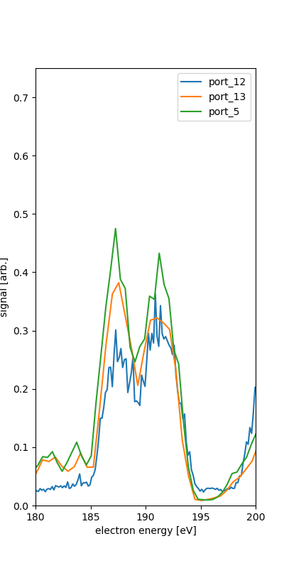
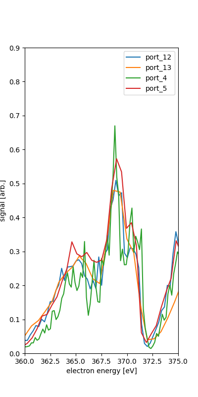
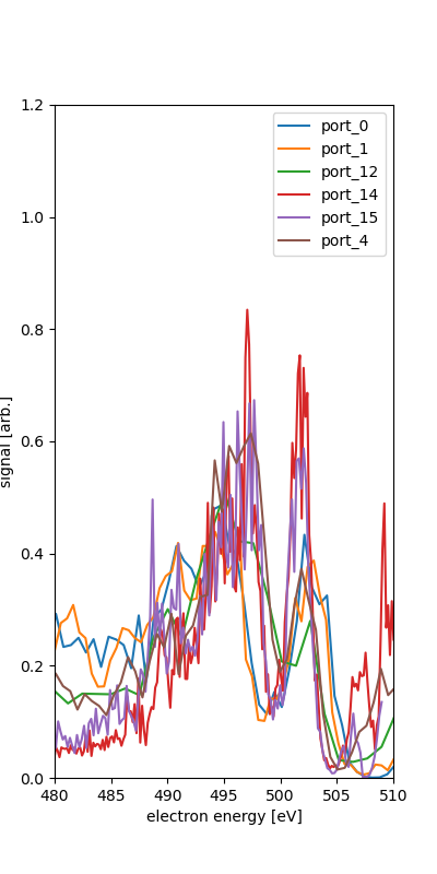
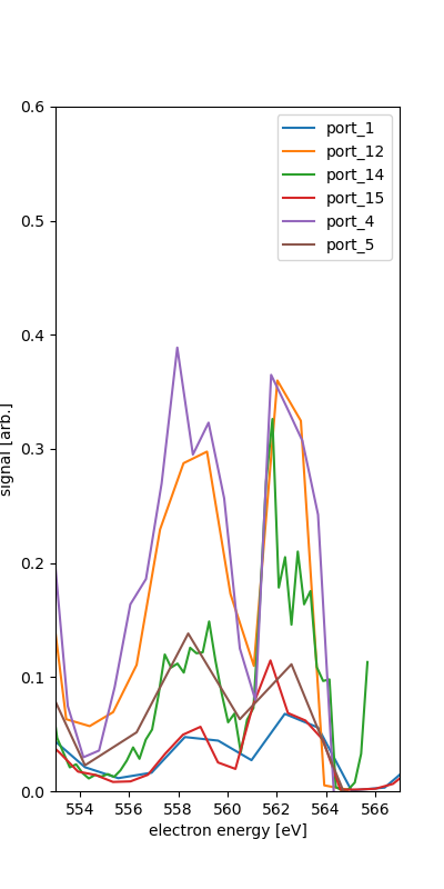
It is clear, here from Run 132 (3rd order VLS spectrum near 600eV photon energy) that the correlation tends to lower photon energy (toward left) for higher x-ray intensity shots.
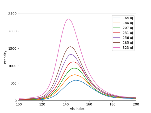
"Knowledge-based quantization (cumsum) reather than a training-based quantization (Berthie)" Audrey Corbeil Therrien Using this src/quantizeGmd.py and figures/plotting.counts.py to make figures related to count rates. So far, the runs e.g. 188 and 189 are grouped into the quantized histogramed .h5 files together with 188... later, do Neon and there only using one run for each set of figures. The count rate looks to be about 1-3 per feature spectral feature.
#Vernier scanning res-Auger N2O ports 0, 1, 12, 14, 15 look pretty good to do in order for plotting with title '0,pi/8,pi/4,3pi/8,pi/2', maybe try using a vector plot in latex.
sbatch -p psanaq --mem-per-cpu=16GB --gpus-per-node=0 --wrap='/cds/home/c/coffee/analysis_2022/x42619/src/hits2h5.py 35000 tmox42619 313 316'
sbatch -p psanaq --mem-per-cpu=16GB --gpus-per-node=0 --wrap='/cds/home/c/coffee/analysis_2022/x42619/src/hits2h5.py 35000 tmox42619 219 220 221 222 223 224 225 226 227 228 229 230 231 232 233 234 235 236 237 238 239 240 241 242'
sbatch -p psanaq --mem-per-cpu=16GB --gpus-per-node=0 --wrap='/cds/home/c/coffee/analysis_2022/x42619/src/hits2h5.py 35000 tmox42619 243 244 245 246'
sbatch -p psanaq --mem-per-cpu=16GB --gpus-per-node=0 --wrap='/cds/home/c/coffee/analysis_2022/x42619/src/hits2h5.py 35000 tmox42619 247 248 249 250 251 252 253 254'
sbatch -p psanaq --mem-per-cpu=16GB --gpus-per-node=0 --wrap='/cds/home/c/coffee/analysis_2022/x42619/src/hits2h5.py 35000 tmox42619 255 256 258 259 260 261 262 263 257'
/cds/home/c/coffee/analysis_2022/x42619/src/quantizeVls.py 256 128 /reg/data/ana16/tmo/tmox42619/scratch/ryan_output_vernier/h5files/hits.tmox42619.run_22[0-5].h5
/cds/home/c/coffee/analysis_2022/x42619/src/quantizeVls.py 256 64 /reg/data/ana16/tmo/tmox42619/scratch/ryan_output_vernier/h5files/hits.tmox42619.run_22[013456789].h5 /reg/data/ana16/tmo/tmox42619/scratch/ryan_output_vernier/h5files/hits.tmox42619.run_24[0-2].h5 /reg/data/ana16/tmo/tmox42619/scratch/ryan_output_vernier/h5files/hits.tmox42619.run_23[2-4].h5
Runs 219-231 are vernier around 532eV-540eV VRET 75V
Runs 232-242 are vernier around 527eV-535eV VRET 75V
Runs 202-206 are at 450 VRET marchine 545-540eV photons, then 207-218 are 450V retardation with vernier, use these for Augers.
Runs 187-200 are 0 VRET but marching down from 575eV-545eV photons, VLS should be fixed.
Runs 169-182 the VLSpitch was different, but 600eV photons for retardations from 0V to 55V.
#Non-vernier scans in Neon
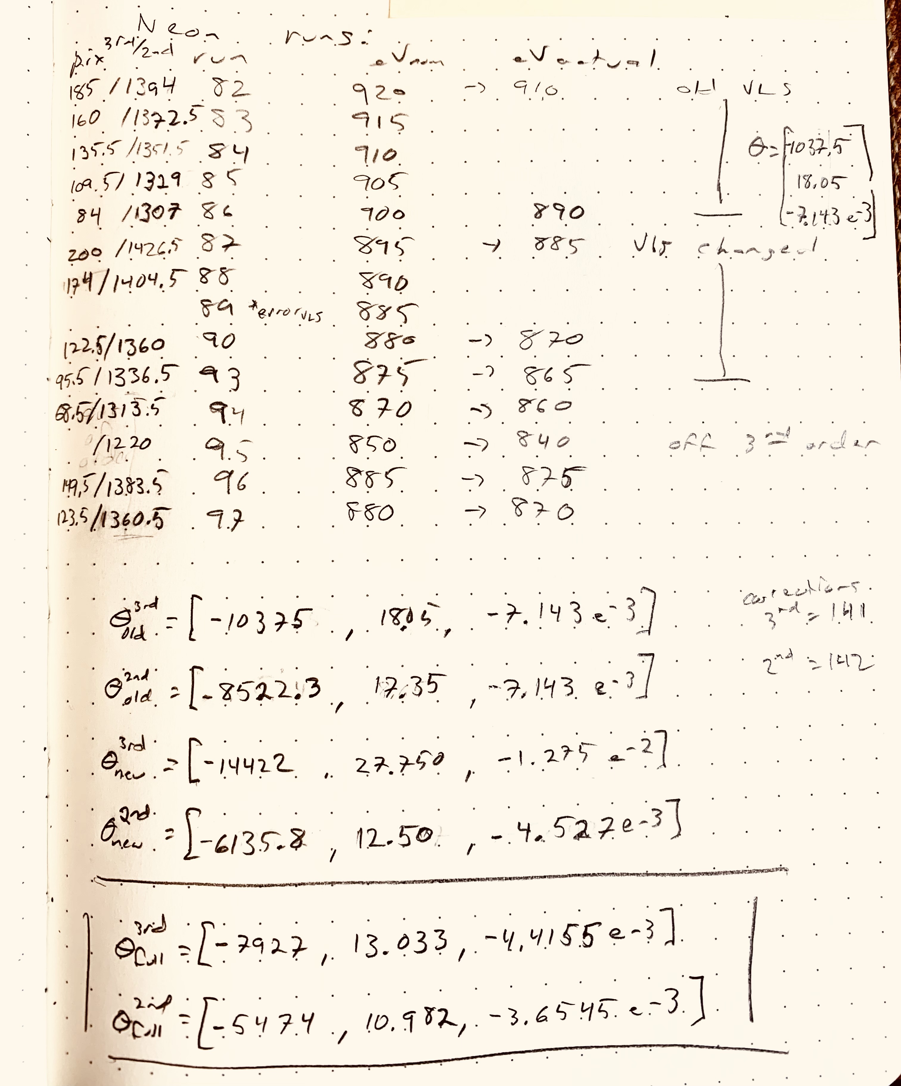 Ugh... need to compute centroids for Neon only above 1000, or alternatively below 512 on VLS except for run 95 which was lowers 850eV photon energy.
82-86 have VLS-pitch 6.9, but 87-90,93-97 use VLS-pitch 6.8, so we need to correct for this when sorting on vls centroids.
The vlspitch correct is +141 for 87--on for third order spectrum (below 1024 on andor).
The vlspitch correct is +142 for 87--on for second order spectrum (above 1024 on andor).
I have hardcoded these vls pitch correction into quantizeVls.py.
Mostly this is to get everyone to see we are using very little of the uint16 bit-depth for our waveforms in abaco high sample rate digitizers (hsd).
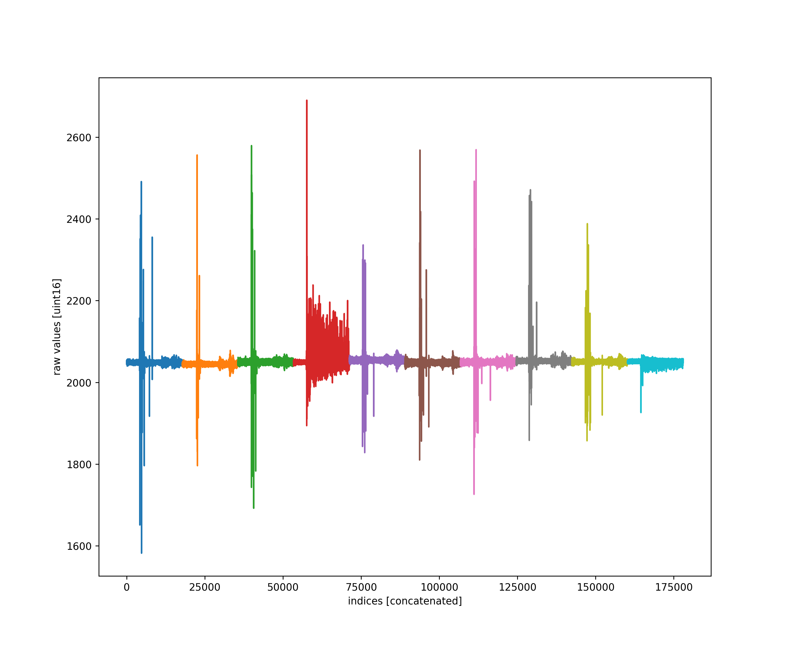
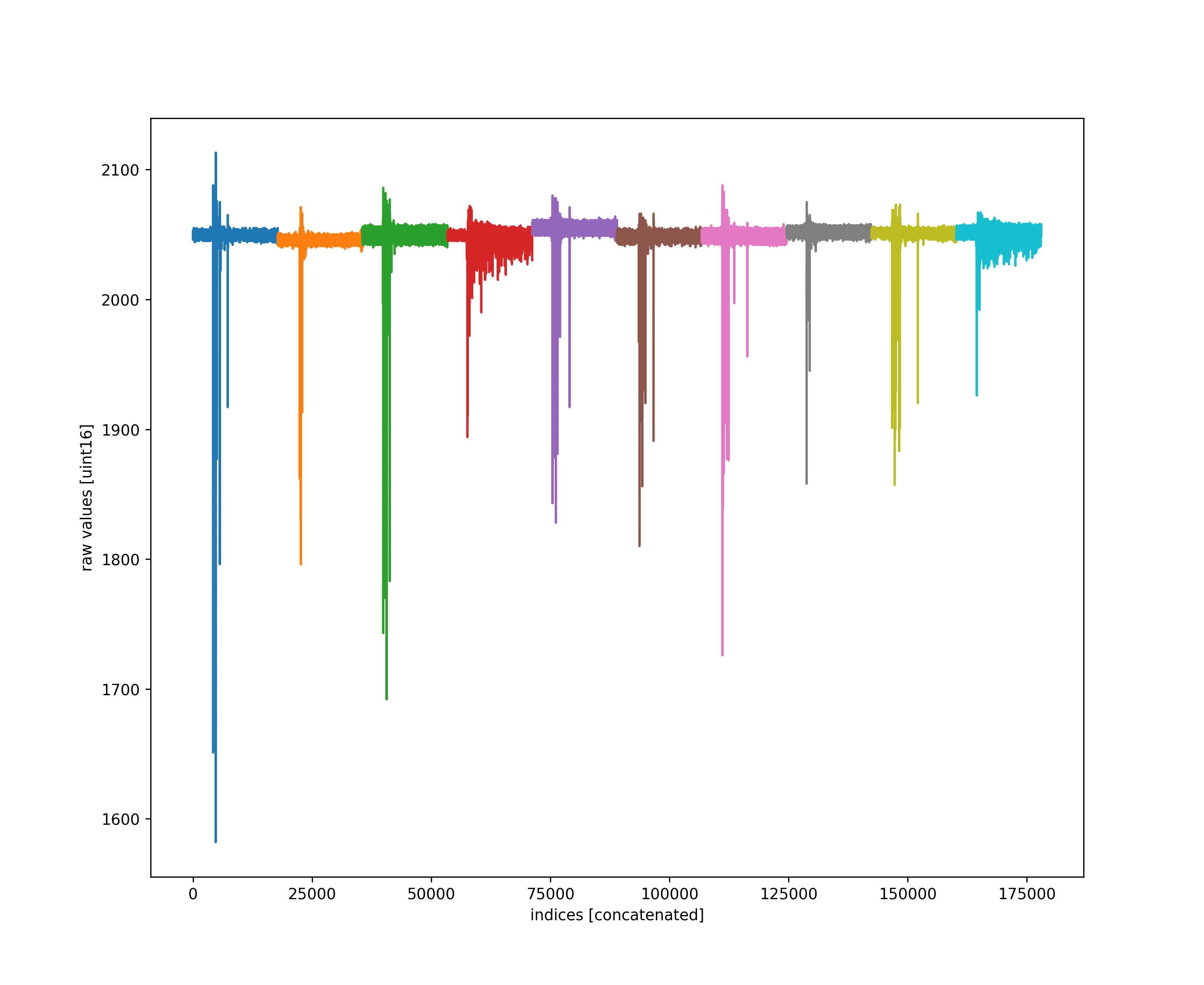
src/waves2h5.py calls processChristos() which adds every raw waveform along with the adc baseline corrected, and the corresponding logic vector.
This is done by including the Port.addeverysample() method to processChristos().
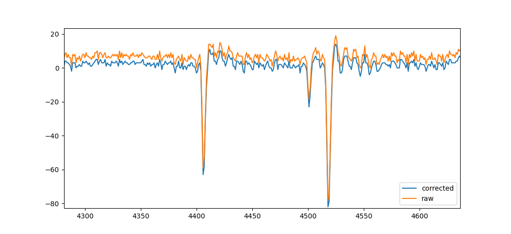 This example is from file
 /reg/data/ana16/tmo/tmox42619/scratch/ryan_output_Christos/h5files/waves.tmox42619.run_084.h5
Hacking the two-color from runs 316 and 313 for Razib SASE reconstruction with Auger.
runs: 313 316 315 314 photon energies:408 404 408 408 rets: 300 300 350 370
Photonenergies 600eV, 500eV, 400eV, 700eV
All 0V retardation: Runs 7 21 36 59
50V retardation: Runs 8 23 39 61
100V retardation: Runs 9 26 42 62
150V retardation: Runs 10 28 -- 63
175V retardation: Runs 11 29 --
Careful, the runs of 100eV different photon energies had different vls pitches, so that needs to be calibrated instead of blindly added as doing now.
Watch it... vls pitch changed between run 86 and 87... careful!
Furthermore, having trouble with evt in run 86 for some reason.
All 0V retardation.
photon energies: 920 915 910 905 [900] 895 890 885 880 875 870 850
runs: 82 83 84 85 [86] 87 88 89 90 93 94 95
vls pitch: 6.9 6.9 6.9 6.9 6.9 6.8 6.8 6.8 6.8 6.8 6.8 6.8
This repo is predominantly for analysis of the lcls x42619 beamtime performed end of June 2021.
This will also host code that analyzes for the xcomm118 for runs in the 400's since that was the commissioning shifts.
First set the configuration .h5 file with something like this...
./src/set_configures.py /reg/data/ana16/tmo/tmox42619/scratch/ryan_output_2022/h5files/tmox42619.hsdconfig.h5Here one must be sure that the file written is indeed what will be read in ./src/hits2h5.py
the expname gets used to pull the config file, at least until we implement the parser.
scratchpath=/reg/data/ana16/tmo/tmox42619/scratch/ryan_output_2022/h5files
expname=tmox42619
runnum=23
shots=100
./src/set_configures.py ${scratchpath}/${expname}.hsdconfig.h5
./src/hits2h5.py ${expname} ${runnum} ${nshots}sbatch -p psanaq --nodes 1 --ntasks-per-node 1 --wrap="./src/hits2h5.py tmox42619 23 10000"
coffee@psanagpu103:x42619$ for id in 21 22 23 25 26 27 28 29 30; do sbatch -p psanaq --nodes 1 --ntasks-per-node 1 --mem-per-cpu=8GB --gpus-per-node=0 --wrap="/cds/home/c/coffee/analysis_2022/x42619/src/hits2h5.py tmox42619 $id 40000"; doneThe first line creates the calibration file based on the hard coded hand calibrated-by ryan values for the argon Auger-Meitner lines near 200-210eV (for 600eV photon energy so far).
The second line then fits those values and writes the resulting quadratic fit to a file 'calibfit.h5'.
./src/argon.calib.auger.py /media/coffee/dataSD/ryan_output_2022/calib/argon.calib.20220411.h5
./src/argon.calib.auger.fitting.py /media/coffee/dataSD/ryan_output_2022/calib/argon.calib.20220411.h5
Inside ./src/argon.calib.auger.fitting.py there are both fit() and transform() methods. These I plan to make compatible with import for post processing the 'tofs' arrays in the hits2h5.py result.
Apr14 The scirpt ./src/apply_calib.py is not finished... still need to output the spectra (histograms) for each of the ports. I left my usual HERE HERE HERE in there to make the code fail there.
OK, this is how I ran before:
for id in 21 22 23 25 26 27 28 29 30; do sbatch -p psanaq --nodes 1 --ntasks-per-node 1 --mem-per-cpu=32GB --gpus-per-node=0 --wrap="/cds/home/c/coffee/analysis_2022/x42619/src/hits2h5.py tmox42619 $id 40000"; doneUse logarithmic eigenvals representaiton,
fit with a low order polynomial for below i = 300 and above.
use the fits to produce a "weiner filter"
Then approximate the weiner filter with a reverse sin() version of the erf()... e.g. 1 if i<icen-w;0 if i>icen+w; otherwise 0.5*( 1.-sin(pi/2*(i-icen)/w) )
this icen+w is also where we truncate the eigvecs, beyond this is out of signal.
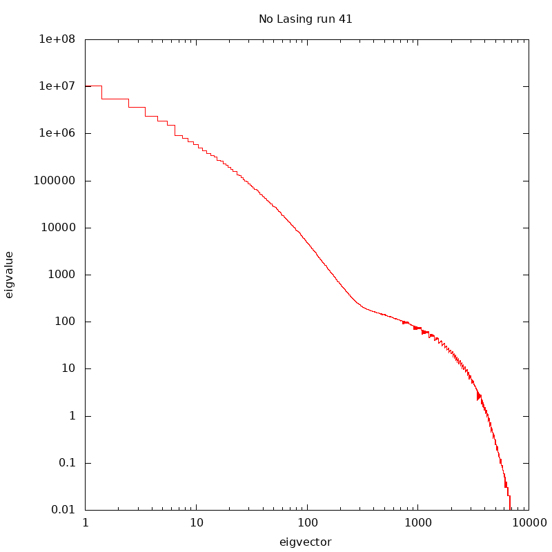 Eigenvalues for Run 41 nolasing
sbatch -p psanaq --nodes 1 --ntasks-per-node 16 --mem-per-cpu=16GB --gpus-per-node=0 --wrap="./src/eigen_xtcav.py /reg/data/ana16/tmo/tmox42619/scratch/ryan_output_2022/h5files/hits.tmox42619.run41.h5 /reg/data/ana16/tmo/tmox42619/scratch/ryan_output_2022/xtcav"