raphael-group/fastBE

fastBE: An ultrafast method for phylogenetic reconstruction from bulk DNA sequencing data

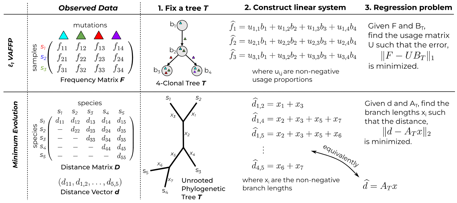
fastBE is a method for inferring the evolutionary history of tumors from multi-sample bulk DNA sequencing data. Our method uses ideas from distance based phylogenetics and a handcrafted solver of the variant allele frequency $\ell_1$-regression problem.

If you find this tool useful in your research, please cite us at:

@article{schmidt2024regression,
  title={A regression based approach to phylogenetic reconstruction from multi-sample bulk DNA sequencing of tumors},
  author={Schmidt, Henri and Raphael, Benjamin J},
  journal={bioRxiv},
  pages={2024--04},
  year={2024},
  publisher={Cold Spring Harbor Laboratory}
}

Installation

Option 1: conda install

To install using conda execute the following command:

$ conda install schmidt73::fastbe

Currently, fastBE is only available through conda for Linux. Additional platforms will be supported upon request.

Option 2: Pre-compiled binaries

Pre-compiled binaries for fastBE are available for both macOS and Linux under the releases section. To install, simply copy the binary into a directory which is recognized by your shell.

Option 3: Build from source

fastBE is implemented in C++ and is packaged with the dependencies needed to execute the program. The only dependencies are a recent version of CMAKE and a modern C++17 compliant compiler.

To build fastBE from source, first clone the repository and its submodules:

$ git clone --recurse-submodules https://github.com/schmidt73/fastbe.git

Then from the root of the project directory, execute the following sequence o commands:

$ mkdir build; cd build
$ cmake ..
$ make

The output binary will be located at build/src/fastbe.

Usage

To run fastbe, simply execute the binary.

$ fastbe
Usage: fastbe [--help] [--version] {regress,search}

Optional arguments:
  -h, --help     shows help message and exits 
  -v, --version  prints version information and exits 

Subcommands:
  regress       Regresses a clone tree onto a frequency matrix.
  search        Searches for a clone tree that best fits a frequency matrix.

The two modes of fastbe are search and regress. The search mode infers the phylogenetic tree best fitting the input frequency matrix, while the regress mode infers the fit of the input tree to the frequency matrix. If one is interested in inferring a phylogenetic tree from a frequency matrix, the search mode should be used.

Formally, the search mode solves the variant allele frequency $\ell_1$-factorization problem, while the regress mode solves the variant allele frequency $\ell_1$-regression problem, both of which are defined in our manuscript. The search mode takes as input an $m \times n$ frequency matrix $F$ and outputs an $n$-clonal tree that best fits the frequency matrix. The regress mode takes as input an $m \times n$ frequency matrix $F$ and an $n$-clonal tree $\mathcal{T}$ and outputs the minimum value of $\lVert F - UB_{\mathcal{T}} \rVert_1$ over all usage matrices $U$.

Important

The search command requires a root vertex specified with the -f/--assigned-root flag, corresponding to the appropriate column of the frequency matrix. By default this root vertex is set to be $0$, or the first column of the frequency matrix. When the root vertex is unknown, it suffices to append an extra column to the beginning of the frequency matrix and specify the root as $0$.

Tip

Use the first column of the frequency matrix as the mutation off the root.

Input format

The input format for the search mode of fastbe consists of a frequency matrix $F$ in .txt format. Rows are separated by newlines and columns are separated by spaces. Rows correspond to distinct samples and columns correspond to distinct mutations (or mutation clusters). More formally, $F_{ij}$ is the frequency of the $j^{\text{th}}$ mutation in the $i^{\text{th}}$ sample. As an example, a frequency matrix $F$ describing $20$ samples and $10$ mutations is:

1.0000 0.9801 0.0000 0.8265 0.0156 0.3683 0.2450 0.1218 0.1260 0.0000
1.0000 1.0000 0.0000 0.1257 0.0000 0.0000 0.0000 0.0000 0.0000 0.1436
1.0000 0.5202 0.0000 0.4053 0.5045 0.0000 0.0000 0.1945 0.0000 0.0000
1.0000 0.3497 0.6616 0.1302 0.0000 0.0000 0.0000 0.1558 0.0000 0.0000
1.0000 0.7233 0.1356 0.5780 0.1640 0.0574 0.0785 0.2873 0.0728 0.1083
1.0000 0.8394 0.0646 0.8530 0.0000 0.0000 0.0000 0.0000 0.0000 0.8353
1.0000 0.1309 0.6547 0.0000 0.0174 0.0000 0.0000 0.0000 0.0000 0.0000
1.0000 0.4203 0.1889 0.0000 0.0000 0.0000 0.0000 0.0000 0.0000 0.0000
1.0000 0.2731 0.1406 0.2768 0.4452 0.0000 0.0000 0.0000 0.0000 0.0000
1.0000 0.5346 0.4651 0.5437 0.0000 0.0000 0.0000 0.1311 0.1069 0.0000
1.0000 0.1043 0.0000 0.1258 0.7614 0.0000 0.0000 0.0566 0.0685 0.0562
1.0000 0.8784 0.0000 0.3935 0.0122 0.0000 0.0124 0.2469 0.2382 0.1668
1.0000 1.0000 0.0000 0.0000 0.0000 0.0000 0.0000 0.0000 0.0000 0.0000
1.0000 0.9163 0.0412 0.8878 0.0348 0.1197 0.1299 0.6229 0.4443 0.0010
1.0000 0.9130 0.0418 0.6500 0.0458 0.0000 0.0000 0.0000 0.0000 0.0000
1.0000 0.8923 0.0000 0.9118 0.0000 0.0000 0.0000 0.9092 0.0000 0.0000
1.0000 0.9318 0.0000 0.9369 0.0704 0.0000 0.0000 0.8478 0.8136 0.0000
1.0000 0.4489 0.3422 0.4024 0.1828 0.0270 0.0000 0.3257 0.3120 0.0350
1.0000 0.9753 0.0000 0.8931 0.0000 0.5100 0.0506 0.0682 0.0000 0.1435
1.0000 1.0000 0.0000 1.0000 0.0000 0.0000 1.0000 0.0000 0.0000 0.0000

The above frequency matrix $F$ is provided as an input file at examples/sim_obs_frequency_matrix.txt.

The input format for the regress mode of fastbe is the aforementioned frequency matrix $F$ and an $n$-clonal tree $\mathcal{T}$. The tree is specified as an adjacency list in .txt format. An example of a clonal tree which consists of $10$ clones rooted at the $0$ vertex is:

The above clonal tree $\mathcal{T}$ is provided as an input file at examples/sim_tree.txt. Each vertex in the adjacency list corresponds to a clone. The name of the vertex corresponds to the index of the mutation in the frequency matrix on the edge leading to the vertex.

The above frequency matrix and clonal tree were generated using the command, python scripts/simulation.py --clones 20 --samples 10 --coverage 100 --seed 0 --mutations 100 --output examples/sim which simulates the evolution of a tumor with $10$ mutation clusters (equivalently, clones) and $20$ samples at a read depth of $100\times$ and $100$ mutations distribution across the $10$ mutation clusters. Several other files such as the mutation to clone mapping, the ground truth usage matrix $U$, clonal matrix $B$, and read count matrices are also provided in the examples/ directory.

Example

As an example, we infer a phylogenetic tree from the simulated data with $20$ samples and $10$ clones. To run fastbe on this data, execute:

fastbe search examples/sim_obs_frequency_matrix.txt -o examples/fastbe

This command will output an adjacency list describing the clonal tree at examples/fastbe_tree.txt and a .json file containing metadata at examples/fastbe_results.json.

Benchmarks

The runtime of fastbe scales as $\mathcal{O}(m)$ with the number $m$ of samples and as $\mathcal{O}(n^4\log^2(n))$ with the number $n$ of mutations. As a reference, we provide the runtime of fastbe on the simulated data with $m = 100$ samples and a varying number of mutations $n$ with default parameters. The system used for benchmarking is an Intel Core i7-8665U CPU @ 1.90GHz × 8 with 8GB of RAM.

Mutations ($n$)	Samples ($m$)	Runtime (s)
10	100	4
25	100	41
50	100	148
100	100	486
200	100	923
500	100	3161
1000	100	4145

The memory footprint of fastbe is $O(mn + nb)$ where $b$ is the beam width for almost all applications. The memory footprint of fastbe is negligible for almost all applications.

When running the search mode of fastbe, the beam width of the search algorithm can be specified with the -b/--beam_width flag. The beam width controls the number of candidate trees that are considered at each iteration of the search algorithm. The runtime of the search algorithm scales approximately linearly with the beam width, and the quality of the inferred tree improves with increased beam width.

Tip

Use the default beam width chosen by fastbe for most applications.

raphael-group / fastBE