In this lesson, you'll learn how to run your first multiple linear regression model using StatsModels.
You will be able to:
- Perform a multiple linear regression using StatsModels
- Visualize individual predictors within a multiple linear regression
- Interpret multiple linear regression coefficients from raw, un-transformed data
The Auto MPG dataset is a classic example of a regression dataset that was first released in 1983.
MPG stands for "miles per gallon", the target to be predicted. There are also several potential independent variables.
import matplotlib.pyplot as plt
import pandas as pd
import statsmodels.api as sm

data = pd.read_csv("auto-mpg.csv")
data.head
<bound method NDFrame.head of mpg cylinders displacement horsepower weight acceleration \
0 18.0 8 307.0 130 3504 12.0
1 15.0 8 350.0 165 3693 11.5
2 18.0 8 318.0 150 3436 11.0
3 16.0 8 304.0 150 3433 12.0
4 17.0 8 302.0 140 3449 10.5
.. ... ... ... ... ... ...
387 27.0 4 140.0 86 2790 15.6
388 44.0 4 97.0 52 2130 24.6
389 32.0 4 135.0 84 2295 11.6
390 28.0 4 120.0 79 2625 18.6
391 31.0 4 119.0 82 2720 19.4
model year origin car name
0 70 1 chevrolet chevelle malibu
1 70 1 buick skylark 320
2 70 1 plymouth satellite
3 70 1 amc rebel sst
4 70 1 ford torino
.. ... ... ...
387 82 1 ford mustang gl
388 82 2 vw pickup
389 82 1 dodge rampage
390 82 1 ford ranger
391 82 1 chevy s-10
[392 rows x 9 columns]>
Let's look at correlations between the other variables and mpg. We need to remove car name since it is categorical.
data = data.drop(columns=['car name'])data.corr()["mpg"]mpg 1.000000
cylinders -0.777618
displacement -0.805127
horsepower -0.778427
weight -0.832244
acceleration 0.423329
model year 0.580541
origin 0.565209
Name: mpg, dtype: float64
Since correlation is a measure related to regression modeling, we can see that there seems to be some relevant signal here, with lots of variables that have medium-to-strong correlations with MPG.
Regression models are evaluated against a "baseline". For simple linear regression, this baseline is an "intercept-only" model that just predicts the mean of the dependent variable every time. For multiple linear regression, we typically build a simple linear regression to be that baseline.
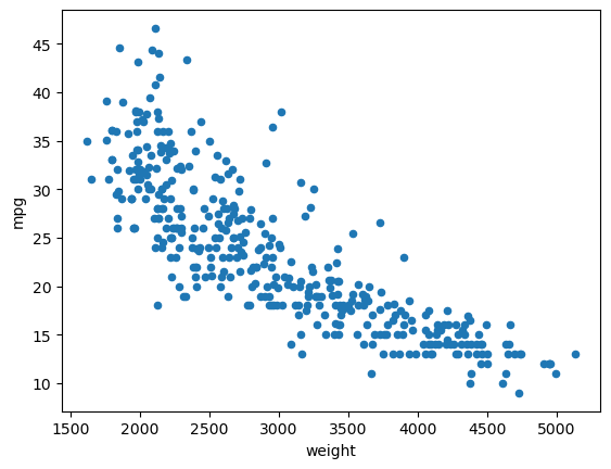
Since weight is the feature with the strongest correlation, let's build a simple linear regression with that.
In other words, we are setting up the formula
Where mpg, the dependent (endogenous) variable, and weight, the independent (exogenous) variable. When we fit our model, we are looking for
data.plot.scatter(x="weight", y="mpg");y = data["mpg"]
X_baseline = data[["weight"]]baseline_model = sm.OLS(y, sm.add_constant(X_baseline))
baseline_results = baseline_model.fit()
print(baseline_results.summary()) OLS Regression Results
==============================================================================
Dep. Variable: mpg R-squared: 0.693
Model: OLS Adj. R-squared: 0.692
Method: Least Squares F-statistic: 878.8
Date: Wed, 19 Jul 2023 Prob (F-statistic): 6.02e-102
Time: 07:58:30 Log-Likelihood: -1130.0
No. Observations: 392 AIC: 2264.
Df Residuals: 390 BIC: 2272.
Df Model: 1
Covariance Type: nonrobust
==============================================================================
coef std err t P>|t| [0.025 0.975]
------------------------------------------------------------------------------
const 46.2165 0.799 57.867 0.000 44.646 47.787
weight -0.0076 0.000 -29.645 0.000 -0.008 -0.007
==============================================================================
Omnibus: 41.682 Durbin-Watson: 0.808
Prob(Omnibus): 0.000 Jarque-Bera (JB): 60.039
Skew: 0.727 Prob(JB): 9.18e-14
Kurtosis: 4.251 Cond. No. 1.13e+04
==============================================================================
Notes:
[1] Standard Errors assume that the covariance matrix of the errors is correctly specified.
[2] The condition number is large, 1.13e+04. This might indicate that there are
strong multicollinearity or other numerical problems.
Looking at the summary above, we can see that the regression line we found was
- The model is statistically significant overall, with an F-statistic p-value well below 0.05
- The model explains about 70% of the variance in MPG
- The model coefficients (
constandweight) are both statistically significant, with t-statistic p-values well below 0.05 - If a car weighed 0 lbs, we would expect MPG to be about 46
- For each increase of 1 lb in car weight, we see an associated decrease in MPG of about .008
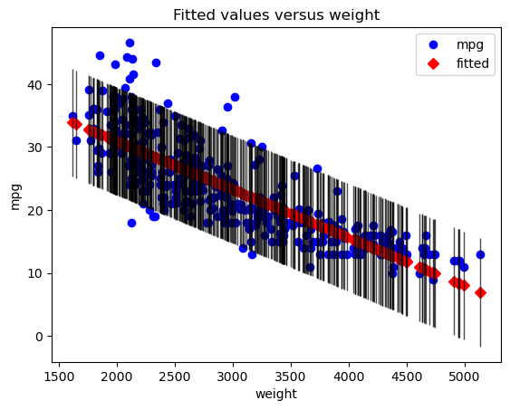
We'll also plot the actual vs. predicted values:
sm.graphics.plot_fit(baseline_results, "weight")
plt.show()
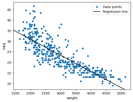
The regression line:
fig, ax = plt.subplots()
data.plot.scatter(x="weight", y="mpg", label="Data points", ax=ax)
sm.graphics.abline_plot(model_results=baseline_results, label="Regression line", ax=ax, color="black")
ax.legend();
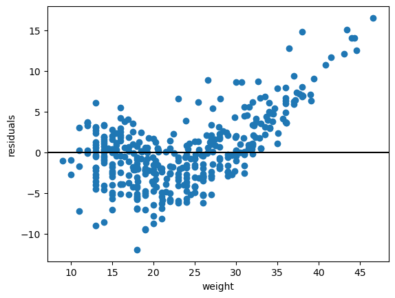
And the residuals:
fig, ax = plt.subplots()

ax.scatter(data["mpg"], baseline_results.resid)
ax.axhline(y=0, color="black")
ax.set_xlabel("weight")
ax.set_ylabel("residuals");Now let's expand from our simple linear regression to a multiple linear regression. It looks like model year is our most strongly positively correlated predictor, so let's add that.
The process of building this model with StatsModels is very similar to the process of building our baseline simple regression model; this time we simply create an X variable containing multiple columns.
X_second = data[["weight", "model year"]]
X_second.dataframe tbody tr th {
vertical-align: top;
}
.dataframe thead th {
text-align: right;
}
| weight | model year | |
|---|---|---|
| 0 | 3504 | 70 |
| 1 | 3693 | 70 |
| 2 | 3436 | 70 |
| 3 | 3433 | 70 |
| 4 | 3449 | 70 |
| ... | ... | ... |
| 387 | 2790 | 82 |
| 388 | 2130 | 82 |
| 389 | 2295 | 82 |
| 390 | 2625 | 82 |
| 391 | 2720 | 82 |
392 rows × 2 columns
second_model = sm.OLS(y, sm.add_constant(X_second))
second_results = second_model.fit()

print(second_results.summary())
OLS Regression Results
==============================================================================
Dep. Variable: mpg R-squared: 0.808
Model: OLS Adj. R-squared: 0.807
Method: Least Squares F-statistic: 819.5
Date: Wed, 19 Jul 2023 Prob (F-statistic): 3.33e-140
Time: 07:58:30 Log-Likelihood: -1037.6
No. Observations: 392 AIC: 2081.
Df Residuals: 389 BIC: 2093.
Df Model: 2
Covariance Type: nonrobust
==============================================================================
coef std err t P>|t| [0.025 0.975]
------------------------------------------------------------------------------
const -14.3473 4.007 -3.581 0.000 -22.224 -6.470
weight -0.0066 0.000 -30.911 0.000 -0.007 -0.006
model year 0.7573 0.049 15.308 0.000 0.660 0.855
==============================================================================
Omnibus: 42.504 Durbin-Watson: 1.230
Prob(Omnibus): 0.000 Jarque-Bera (JB): 71.997
Skew: 0.670 Prob(JB): 2.32e-16
Kurtosis: 4.616 Cond. No. 7.17e+04
==============================================================================
Notes:
[1] Standard Errors assume that the covariance matrix of the errors is correctly specified.
[2] The condition number is large, 7.17e+04. This might indicate that there are
strong multicollinearity or other numerical problems.
This time, the model we built was:
- The model is statistically significant overall, with an F-statistic p-value well below 0.05
- The model explains about 81% of the variance in MPG
- The model coefficients (
const,weight, andmodel year) are all statistically significant, with t-statistic p-values well below 0.05 - For each increase of 1 lb in car weight, we see an associated decrease in MPG of about .007
- This is a little bit smaller of a decrease than we saw with the simple model, but not a big change. This means that model year was not meaningfully confounding in the relationship between weight and MPG
- For each increase of 1 in the model year, we see an associated increase in MPG of about 0.76
Notice that the const coefficient has gone from a positive number to a negative number. This is because the intercept is now with respect to both the weight and the model year. How should we interpret a value of zero for model year?
data["model year"].value_counts(sort=False)model year
70 29
71 27
72 28
73 40
74 26
75 30
76 34
77 28
78 36
79 29
80 27
81 28
82 30
Name: count, dtype: int64
Since we know this is a dataset from 1983, it is reasonable to assume that these represent years from 1970 to 1982. Therefore a zero for model year means 1900.
Thus our intercept of about -14.3 means that our model predicts that a car released in 1900 that weighed 0 lbs would have an MPG of -14.3. This is fairly nonsensical, but some intercept is needed to build a linear model. Don't worry too much about trying to draw insights from this value.
We could try to make a 3D plot to show the plane that our model represents. However a more conventional (and extensible) approach is to use several different plots to show different perspectives on the model.
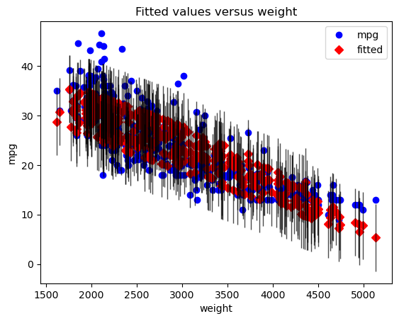
sm.graphics.plot_fit(second_results, "weight")
plt.show()
This shows the true (blue) vs. predicted (red) values, with the particular predictor (in this case, weight) along the x-axis. Note that unlike with a simple regression, the red dots don't appear in a perfectly straight line. This is because their predictions are made based on the entire model, not just this predictor.
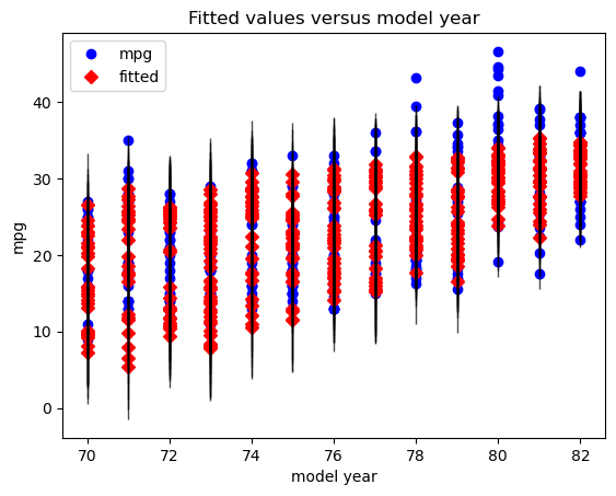
We can also plot the fit for the other predictor, model year:
sm.graphics.plot_fit(second_results, "model year")
plt.show()Then, instead of a basic scatter plot with a best-fit line (since our model is now higher-dimensional), we'll use two partial regression plots, one for each of our predictors.
fig = plt.figure(figsize=(15,5))
sm.graphics.plot_partregress_grid(second_results, exog_idx=["weight", "model year"], fig=fig)
plt.tight_layout()
plt.show()
This may initially appear similar to the plotted regression line from our simple linear regression example, but it is not actually showing the predictor value on the x-axis vs. the target value on the y-axis. Instead, the goal is to show the marginal contribution of this particular predictor.
First let's focus on the left side, which shows the partial regression plot for weight.
The math behind this is that StatsModels has computed the part of weight that is not explained by the rest of the model, and put it on the x-axis. Then it has computed the part of mpg that is not explained by the rest of the model, and put it on the y-axis. If this plot shows a linear relationship with a non-zero slope, that means that it is beneficial to add weight to the model, vs. having a model without weight (i.e. a model with just an intercept and model year).
The partial regression plot for model year is similarly showing the marginal contribution of model year compared to a model with just weight.
A reasonable conclusion to reach, looking at these plots, is that both predictors are useful and should be included in the model.
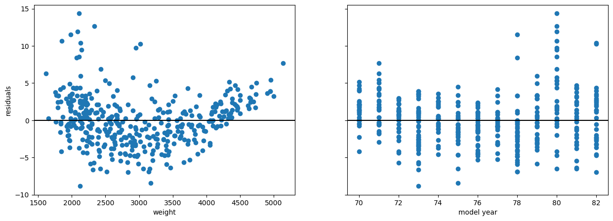
One approach to plotting residuals from a multiple regression model is to use the same approach as in simple regression, just plotting the value of the predictor on the x-axis vs. the model residuals on the y-axis.
fig, axes = plt.subplots(ncols=2, figsize=(15,5), sharey=True)

weight_ax = axes[0]
weight_ax.scatter(data["weight"], second_results.resid)
weight_ax.axhline(y=0, color="black")
weight_ax.set_xlabel("weight")
weight_ax.set_ylabel("residuals")

year_ax = axes[1]
year_ax.scatter(data["model year"], second_results.resid)
year_ax.axhline(y=0, color="black")
year_ax.set_xlabel("model year");
Another approach is using a component and component-plus-residual plot, also known as a CCPR plot. A CCPR plot is a refinement of a partial residual plot. A partial residual plot is a scatter plot with the predictor on the x-axis and the model residuals plus the predictor times its coefficient on the y-axis. Then the CCPR plot also includes a line representing the fitted line of the predictor times its coefficient. Similar to a partial regression plot, you are essentially looking for the points and best-fit line to match up and form a linear relationship with non-zero slope.
fig = plt.figure(figsize=(15,5))
sm.graphics.plot_ccpr_grid(second_results, exog_idx=["weight", "model year"], grid=(1,2), fig=fig)
plt.tight_layout()
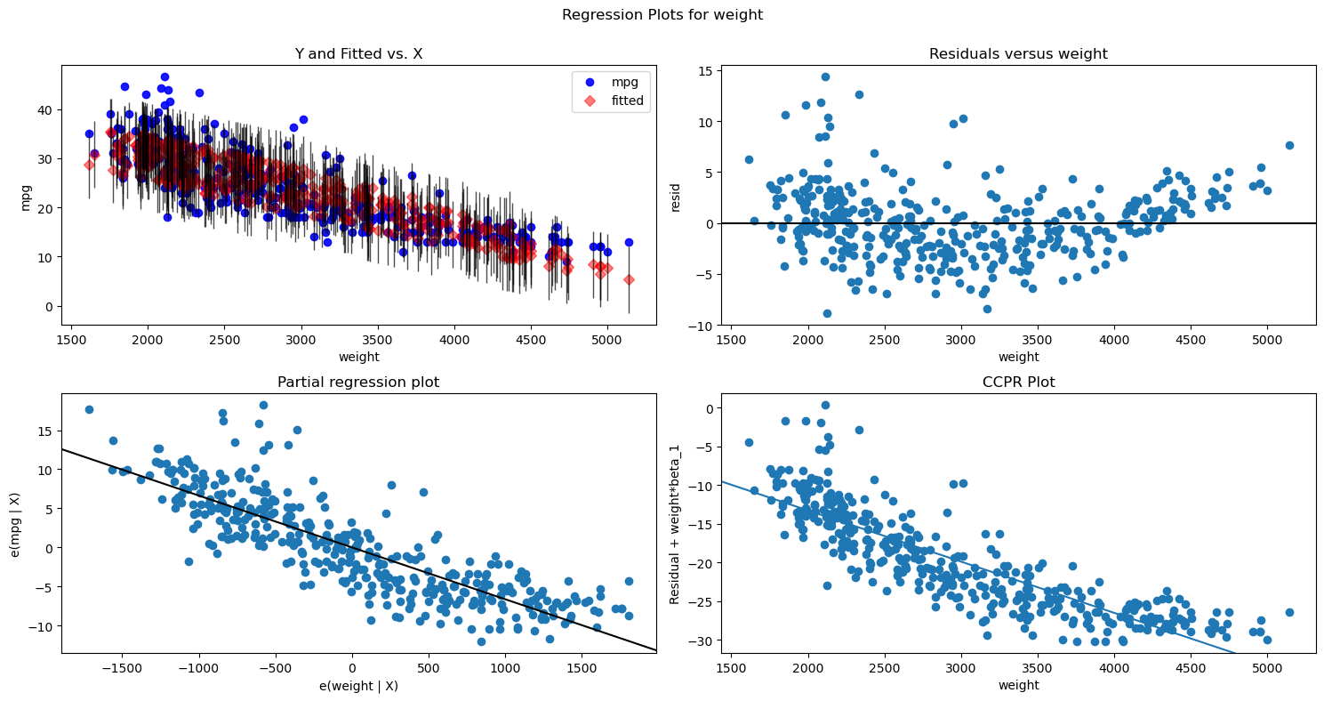
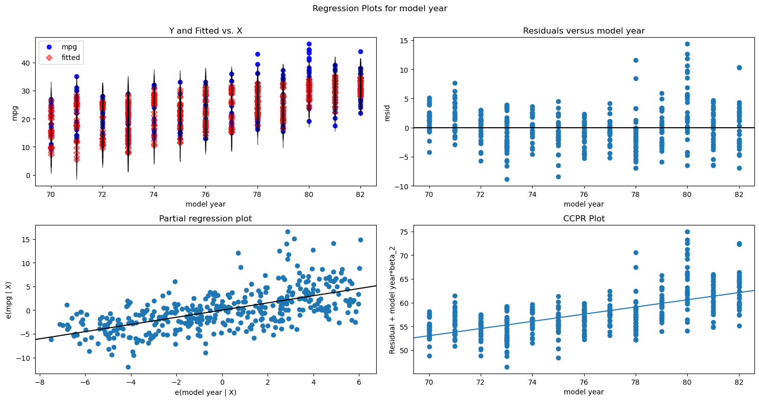
plt.show()If you are interested in creating all of these plots at once for a given predictor, StatsModels has a wrapper that can do this also:
fig = plt.figure(figsize=(15,8))
sm.graphics.plot_regress_exog(second_results, "weight", fig=fig)
plt.show()
fig = plt.figure(figsize=(15,8))
sm.graphics.plot_regress_exog(second_results, "model year", fig=fig)
plt.show()Now that we have a model with 1 predictor (weight) as well as a model with 2 predictors (weight and model year), let's try a model that uses all of the available numeric columns as features.
# dropping mpg because this is our target, then only selecting numeric features
X_all = data.drop("mpg", axis=1).select_dtypes("number")
X_all.dataframe tbody tr th {
vertical-align: top;
}
.dataframe thead th {
text-align: right;
}
| cylinders | displacement | horsepower | weight | acceleration | model year | origin | |
|---|---|---|---|---|---|---|---|
| 0 | 8 | 307.0 | 130 | 3504 | 12.0 | 70 | 1 |
| 1 | 8 | 350.0 | 165 | 3693 | 11.5 | 70 | 1 |
| 2 | 8 | 318.0 | 150 | 3436 | 11.0 | 70 | 1 |
| 3 | 8 | 304.0 | 150 | 3433 | 12.0 | 70 | 1 |
| 4 | 8 | 302.0 | 140 | 3449 | 10.5 | 70 | 1 |
| ... | ... | ... | ... | ... | ... | ... | ... |
| 387 | 4 | 140.0 | 86 | 2790 | 15.6 | 82 | 1 |
| 388 | 4 | 97.0 | 52 | 2130 | 24.6 | 82 | 2 |
| 389 | 4 | 135.0 | 84 | 2295 | 11.6 | 82 | 1 |
| 390 | 4 | 120.0 | 79 | 2625 | 18.6 | 82 | 1 |
| 391 | 4 | 119.0 | 82 | 2720 | 19.4 | 82 | 1 |
392 rows × 7 columns
third_model = sm.OLS(y, sm.add_constant(X_all))
third_results = third_model.fit()

print(third_results.summary())
OLS Regression Results
==============================================================================
Dep. Variable: mpg R-squared: 0.821
Model: OLS Adj. R-squared: 0.818
Method: Least Squares F-statistic: 252.4
Date: Wed, 19 Jul 2023 Prob (F-statistic): 2.04e-139
Time: 07:58:31 Log-Likelihood: -1023.5
No. Observations: 392 AIC: 2063.
Df Residuals: 384 BIC: 2095.
Df Model: 7
Covariance Type: nonrobust
================================================================================
coef std err t P>|t| [0.025 0.975]
--------------------------------------------------------------------------------
const -17.2184 4.644 -3.707 0.000 -26.350 -8.087
cylinders -0.4934 0.323 -1.526 0.128 -1.129 0.142
displacement 0.0199 0.008 2.647 0.008 0.005 0.035
horsepower -0.0170 0.014 -1.230 0.220 -0.044 0.010
weight -0.0065 0.001 -9.929 0.000 -0.008 -0.005
acceleration 0.0806 0.099 0.815 0.415 -0.114 0.275
model year 0.7508 0.051 14.729 0.000 0.651 0.851
origin 1.4261 0.278 5.127 0.000 0.879 1.973
==============================================================================
Omnibus: 31.906 Durbin-Watson: 1.309
Prob(Omnibus): 0.000 Jarque-Bera (JB): 53.100
Skew: 0.529 Prob(JB): 2.95e-12
Kurtosis: 4.460 Cond. No. 8.59e+04
==============================================================================
Notes:
[1] Standard Errors assume that the covariance matrix of the errors is correctly specified.
[2] The condition number is large, 8.59e+04. This might indicate that there are
strong multicollinearity or other numerical problems.
This time, the model we built was:
- The model is statistically significant overall, with an F-statistic p-value well below 0.05
- The model explains about 82% of the variance in MPG
- The fact that we went from 2 predictors to 7 predictors and only increased R-Squared by 1% is an indicator that this is not a very good model
- Only some of the model coefficients are statistically significant
const,displacement,weight,model year, andoriginhave p-values below 0.05 and are therefore statistically significantcylinders,horsepower, andaccelerationhave p-values above 0.05. This means that there is greater than a 1 in 20 chance that their true coefficients are 0 (i.e. they have no effect on MPG), and are thus not statistically significant at an alpha of 0.05
We could go through and interpret the coefficients as well, but for now we'll skip that because there are so many that are not statistically significant.
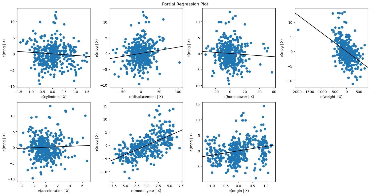
If we ran plot_regress_exog on each of our predictors, that would be 28 different plots -- probably too many to draw any useful conclusions from. Instead, let's plot just the partial regression plots:
fig = plt.figure(figsize=(15,8))
sm.graphics.plot_partregress_grid(
    third_results,
    exog_idx=list(X_all.columns.values),
    grid=(2,4),
    fig=fig)
plt.show()
As you can see, as we have added more predictors, the partial regression plot for each individual one is looking worse. Other than model year and origin, we're seeing more of a cluster of dots rather than a clean linear relationship. We also see that several of them have slopes near zero.
A reasonable interpretation from these visualizations overall is that we have included too many predictors, and that we should consider removing some. We'll discuss more details on feature selection (techniques for deciding which features to include) in future lessons.
StatsModels is only one of several libraries that have implemented linear regression. Another library with linear regression is called scikit-learn.
Scikit-learn is known for its machine learning functionality and is generally very popular for data science workflows. In particular, scikit-learn emphasizes predictive machine learning approaches. Therefore it does not automatically calculate anything related to statistical significance (e.g. p-values), it only calculates the model parameters.
For a comparison of scikit-learn and statsmodels click here.
from sklearn.linear_model import LinearRegressionFirst, let's recreate our baseline model:
sklearn_baseline_model = LinearRegression()
# passing in the same X and y, although the order is reversed
sklearn_baseline_model.fit(X_baseline, y)

print(f"""
StatsModels R-Squared:    {baseline_results.rsquared}
scikit-learn R-Squared:   {sklearn_baseline_model.score(X_baseline, y)}

StatsModels intercept:    {baseline_results.params["const"]}
scikit-learn intercept:   {sklearn_baseline_model.intercept_}

StatsModels coefficient:  {baseline_results.params["weight"]}
scikit-learn coefficient: {sklearn_baseline_model.coef_[0]}
""")
StatsModels R-Squared: 0.6926304331206254
scikit-learn R-Squared: 0.6926304331206254
StatsModels intercept: 46.216524549017585
scikit-learn intercept: 46.21652454901757
StatsModels coefficient: -0.0076473425357795775
scikit-learn coefficient: -0.0076473425357795775
Then our model with two features:
sklearn_second_model = LinearRegression()
sklearn_second_model.fit(X_second, y)

print(f"""
StatsModels R-Squared:    {second_results.rsquared}
scikit-learn R-Squared:   {sklearn_second_model.score(X_second, y)}

StatsModels intercept:     {second_results.params["const"]}
scikit-learn intercept:    {sklearn_second_model.intercept_}

StatsModels coefficients:  {second_results.params[1:].values}
scikit-learn coefficients: {sklearn_second_model.coef_}
""")
StatsModels R-Squared: 0.8081803058793997
scikit-learn R-Squared: 0.8081803058793997
StatsModels intercept: -14.347253017615827
scikit-learn intercept: -14.34725301761586
StatsModels coefficients: [-0.00663208 0.75731828]
scikit-learn coefficients: [-0.00663208 0.75731828]
Then finally our model with all numeric features:
sklearn_third_model = LinearRegression()
sklearn_third_model.fit(X_all, y)

print(f"""
StatsModels R-Squared:    {third_results.rsquared}
scikit-learn R-Squared:   {sklearn_third_model.score(X_all, y)}

StatsModels intercept:     {third_results.params["const"]}
scikit-learn intercept:    {sklearn_third_model.intercept_}

StatsModels coefficients:  {third_results.params[1:].values}
scikit-learn coefficients: {sklearn_third_model.coef_}
""")
StatsModels R-Squared: 0.8214780764810599
scikit-learn R-Squared: 0.8214780764810599
StatsModels intercept: -17.21843462201798
scikit-learn intercept: -17.218434622017558
StatsModels coefficients: [-0.49337632 0.01989564 -0.01695114 -0.00647404 0.08057584 0.75077268
1.4261405 ]
scikit-learn coefficients: [-0.49337632 0.01989564 -0.01695114 -0.00647404 0.08057584 0.75077268
1.4261405 ]
The purpose of this demonstration is so that you can see how StatsModels is just one way of representing a linear regression model with code. Different libraries will use different formats for setting up the x and y values and different formats for displaying the results, but they are fundamentally using the same algorithm "under the hood". As you learn about more types of models and more libraries that represent these models, you do not have to memorize the syntax for using them! Instead, so long as you understand the underlying concepts, you can always refer to the documentation to figure out how a given library represents the modeling process.
Creating multiple linear regression models in StatsModels is very similar to creating simple linear regression models. The only difference is that you supply an x variable containing multiple features instead of just one. In this lesson you saw examples of multiple regression models as well as interpretations of their metrics and coefficients. You also saw some visualization techniques that we use to inspect model fit and residuals in the context of a linear regression model with multiple predictors.
