coronavirus

The coronavirus package provides a tidy format dataset of the 2019 Novel Coronavirus COVID-19 (2019-nCoV) epidemic. The raw data pulled from the Johns Hopkins University Center for Systems Science and Engineering (JHU CCSE) Coronavirus repository.

More details available here, and a csv format of the package dataset available here

A summary dashboard is available here

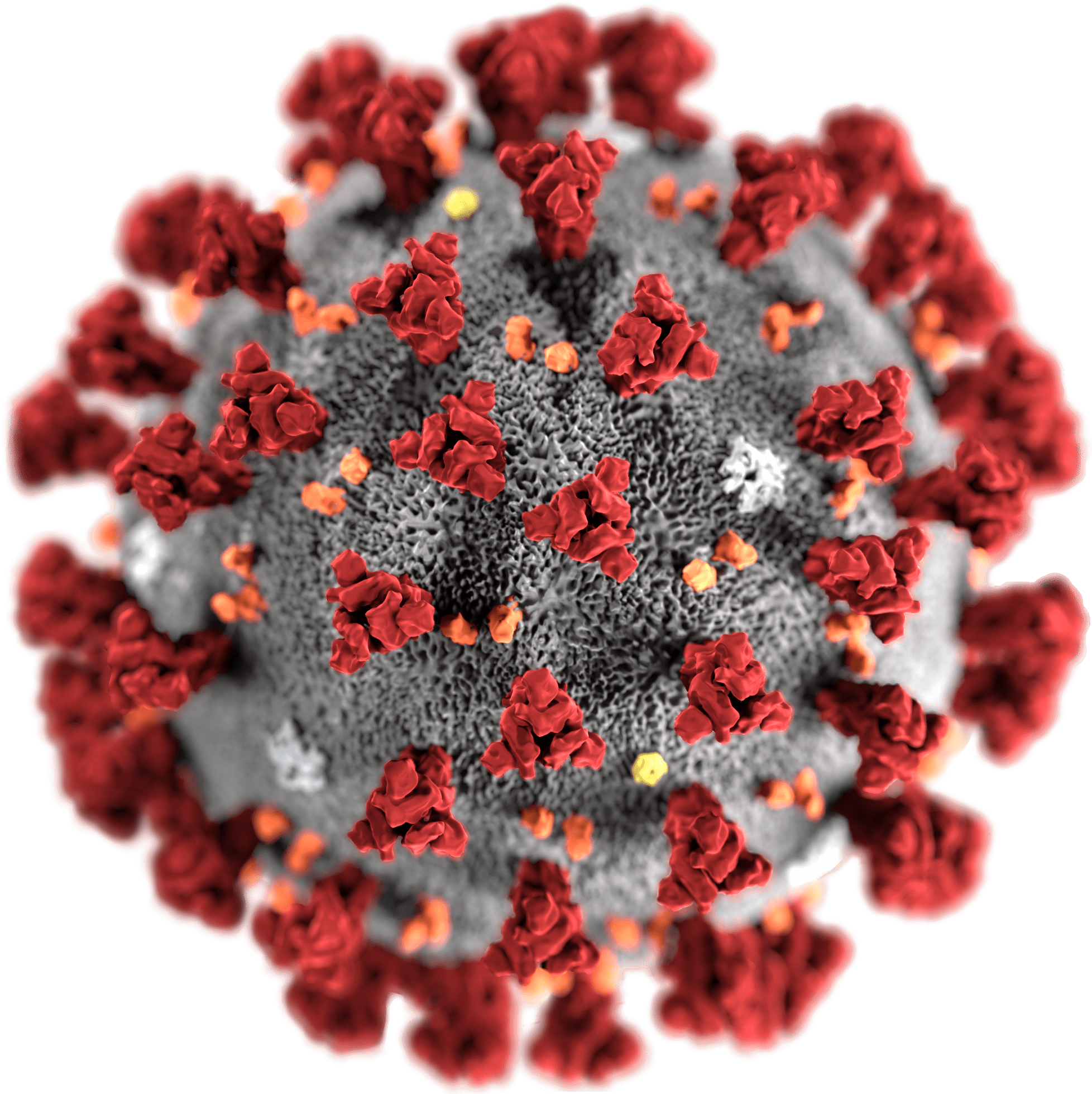
Source: Centers for Disease Control and Prevention’s Public Health Image Library

Important Note

As this an ongoing situation, frequent changes in the data format may occur, please visit the package news to get updates about those changes

Installation

Install the CRAN version:

install.packages("coronavirus")

Install the Github version (refreshed on a daily bases):

# install.packages("devtools")
devtools::install_github("RamiKrispin/coronavirus")

Data refresh

While the coronavirus CRAN version is updated every month or two, the Github (Dev) version is updated on a daily bases. The update_dataset function enables to overcome this gap and keep the installed version with the most recent data available on the Github version:

library(coronavirus)
update_dataset()

Note: must restart the R session to have the updates available

Usage

data("coronavirus")

This coronavirus dataset has the following fields:

date - The date of the summary
province - The province or state, when applicable
country - The country or region name
lat - Latitude point
long - Longitude point
type - the type of case (i.e., confirmed, death)
cases - the number of daily cases (corresponding to the case type)

head(coronavirus)
#>         date province     country lat long      type cases
#> 1 2020-01-22          Afghanistan  33   65 confirmed     0
#> 2 2020-01-23          Afghanistan  33   65 confirmed     0
#> 3 2020-01-24          Afghanistan  33   65 confirmed     0
#> 4 2020-01-25          Afghanistan  33   65 confirmed     0
#> 5 2020-01-26          Afghanistan  33   65 confirmed     0
#> 6 2020-01-27          Afghanistan  33   65 confirmed     0

Summary of the total confrimed cases by country (top 20):

library(dplyr)

summary_df <- coronavirus %>% 
  filter(type == "confirmed") %>%
  group_by(country) %>%
  summarise(total_cases = sum(cases)) %>%
  arrange(-total_cases)

summary_df %>% head(20) 
#> # A tibble: 20 x 2
#>    country        total_cases
#>    <chr>                <int>
#>  1 US                 1369376
#>  2 Russia              232243
#>  3 Spain               228030
#>  4 United Kingdom      227741
#>  5 Italy               221216
#>  6 France              178349
#>  7 Brazil              178214
#>  8 Germany             173171
#>  9 Turkey              141475
#> 10 Iran                110767
#> 11 China                84018
#> 12 India                74292
#> 13 Canada               72419
#> 14 Peru                 72059
#> 15 Belgium              53779
#> 16 Netherlands          43183
#> 17 Saudi Arabia         42925
#> 18 Mexico               38324
#> 19 Pakistan             34336
#> 20 Chile                31721

Summary of new cases during the past 24 hours by country and type (as of 2020-05-12):

library(tidyr)

coronavirus %>% 
  filter(date == max(date)) %>%
  select(country, type, cases) %>%
  group_by(country, type) %>%
  summarise(total_cases = sum(cases)) %>%
  pivot_wider(names_from = type,
              values_from = total_cases) %>%
  arrange(-confirmed)
#> # A tibble: 187 x 4
#> # Groups:   country [187]
#>    country              confirmed death recovered
#>    <chr>                    <int> <int>     <int>
#>  1 US                       21495  1674     -2446
#>  2 Russia                   10899   107      3711
#>  3 Brazil                    8620   808      5213
#>  4 India                     3524   121      1871
#>  5 United Kingdom            3409   628         8
#>  6 Peru                      3237    96       918
#>  7 Pakistan                  2255    31       257
#>  8 Mexico                    1997   353      2835
#>  9 Saudi Arabia              1911     9      2520
#> 10 Turkey                    1704    53      3109
#> 11 Chile                     1658    12       520
#> 12 Qatar                     1526     0       179
#> 13 Iran                      1481    48       935
#> 14 Italy                     1402   172      2452
#> 15 Canada                    1155   185      1048
#> 16 Kuwait                     991    10       194
#> 17 Bangladesh                 969    11       245
#> 18 Belarus                    967     7       443
#> 19 Ecuador                    910   182         0
#> 20 Singapore                  849     0       626
#> 21 France                     802   348      1063
#> 22 United Arab Emirates       783     2       631
#> 23 South Africa               698     0         0
#> 24 Colombia                   659    14       146
#> 25 Sweden                     602    57         0
#> 26 Germany                    595    77      1583
#> 27 Poland                     595    28       315
#> 28 Spain                      594   176      1841
#> 29 Indonesia                  484    16       182
#> 30 Ghana                      427     0         0
#> 31 Ukraine                    375    17        85
#> 32 Egypt                      347    11       154
#> 33 Belgium                    330    54        35
#> 34 Bahrain                    295     1        40
#> 35 Argentina                  285     5        25
#> 36 Afghanistan                276     5        52
#> 37 Dominican Republic         266     9       351
#> 38 Philippines                264    25       107
#> 39 Portugal                   234    19       464
#> 40 Netherlands                196    54         0
#> # … with 147 more rows

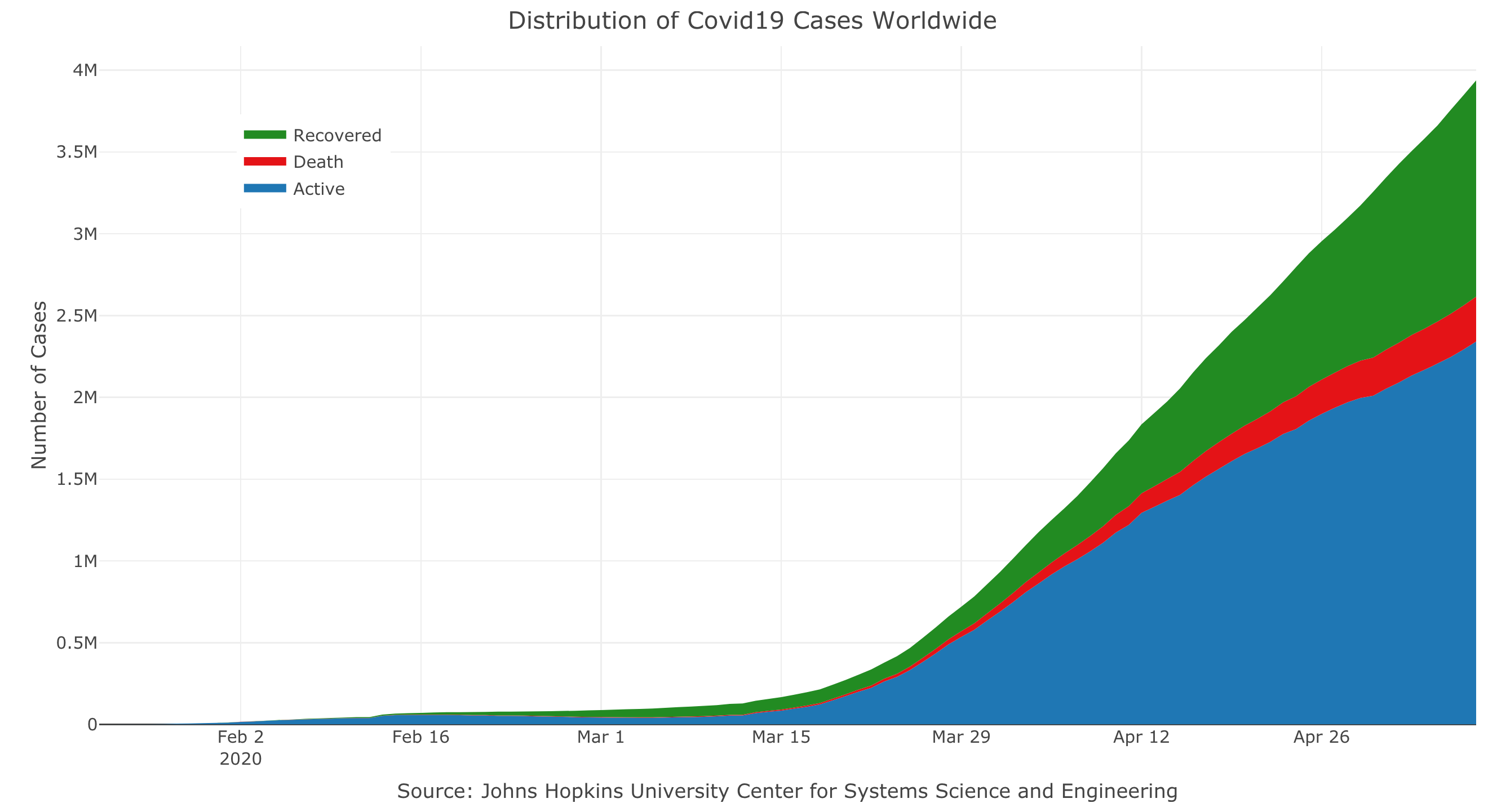
Plotting the total cases by type worldwide:

library(plotly)

coronavirus %>% 
  group_by(type, date) %>%
  summarise(total_cases = sum(cases)) %>%
  pivot_wider(names_from = type, values_from = total_cases) %>%
  arrange(date) %>%
  mutate(active = confirmed - death - recovered) %>%
  mutate(active_total = cumsum(active),
                recovered_total = cumsum(recovered),
                death_total = cumsum(death)) %>%
  plot_ly(x = ~ date,
                  y = ~ active_total,
                  name = 'Active', 
                  fillcolor = '#1f77b4',
                  type = 'scatter',
                  mode = 'none', 
                  stackgroup = 'one') %>%
  add_trace(y = ~ death_total, 
             name = "Death",
             fillcolor = '#E41317') %>%
  add_trace(y = ~recovered_total, 
            name = 'Recovered', 
            fillcolor = 'forestgreen') %>%
  layout(title = "Distribution of Covid19 Cases Worldwide",
         legend = list(x = 0.1, y = 0.9),
         yaxis = list(title = "Number of Cases"),
         xaxis = list(title = "Source: Johns Hopkins University Center for Systems Science and Engineering"))

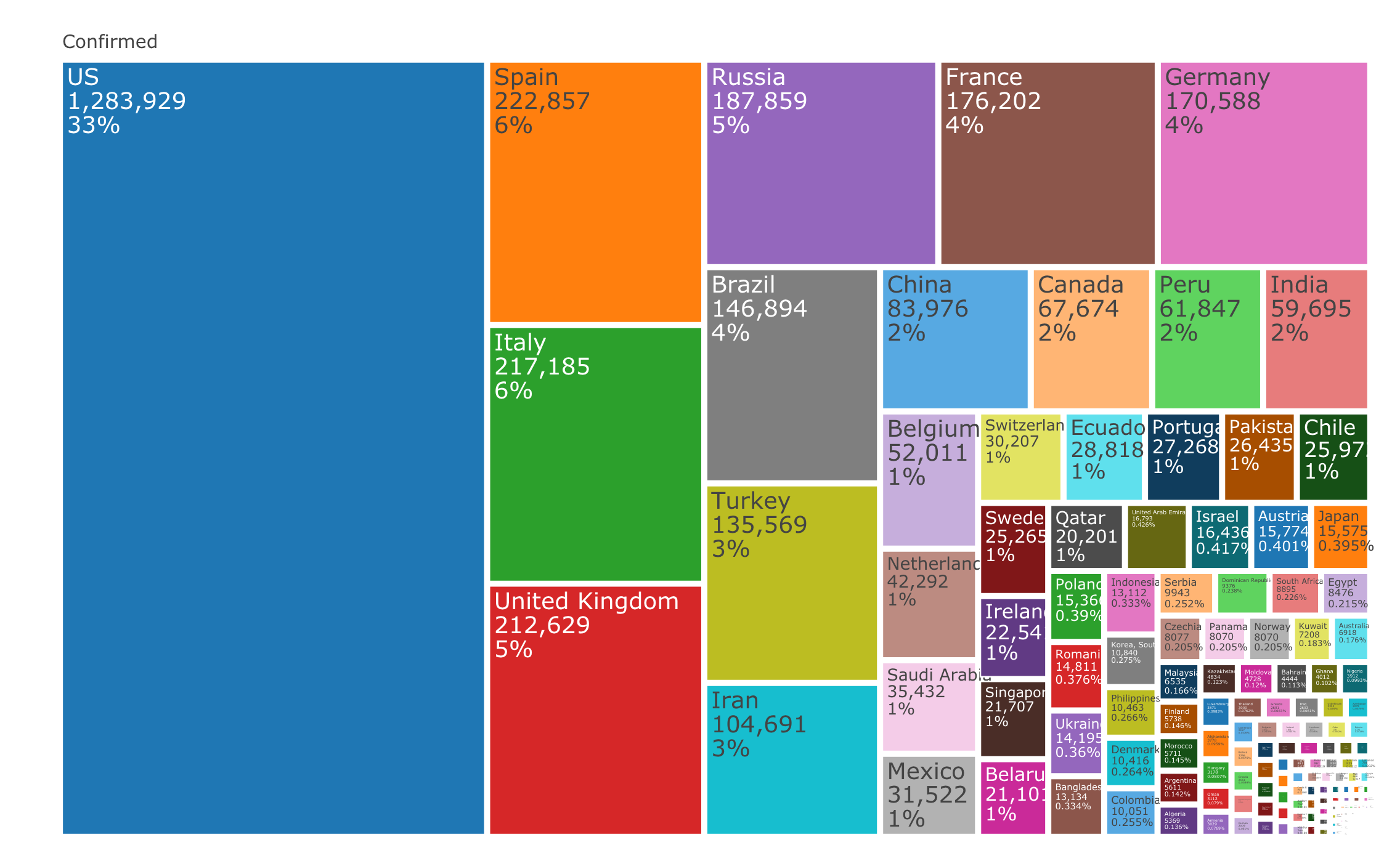
Plot the confirmed cases distribution by counrty with treemap plot:

conf_df <- coronavirus %>% 
  filter(type == "confirmed") %>%
  group_by(country) %>%
  summarise(total_cases = sum(cases)) %>%
  arrange(-total_cases) %>%
  mutate(parents = "Confirmed") %>%
  ungroup() 
  
  plot_ly(data = conf_df,
          type= "treemap",
          values = ~total_cases,
          labels= ~ country,
          parents=  ~parents,
          domain = list(column=0),
          name = "Confirmed",
          textinfo="label+value+percent parent")

Data Sources

The raw data pulled and arranged by the Johns Hopkins University Center for Systems Science and Engineering (JHU CCSE) from the following resources:

World Health Organization (WHO): https://www.who.int/
DXY.cn. Pneumonia. 2020. http://3g.dxy.cn/newh5/view/pneumonia.
BNO News: https://bnonews.com/index.php/2020/02/the-latest-coronavirus-cases/
National Health Commission of the People’s Republic of China (NHC):
http:://www.nhc.gov.cn/xcs/yqtb/list_gzbd.shtml
China CDC (CCDC): http:://weekly.chinacdc.cn/news/TrackingtheEpidemic.htm
Hong Kong Department of Health: https://www.chp.gov.hk/en/features/102465.html
Macau Government: https://www.ssm.gov.mo/portal/
Taiwan CDC: https://sites.google.com/cdc.gov.tw/2019ncov/taiwan?authuser=0
US CDC: https://www.cdc.gov/coronavirus/2019-ncov/index.html
Government of Canada: https://www.canada.ca/en/public-health/services/diseases/coronavirus.html
Australia Government Department of Health: https://www.health.gov.au/news/coronavirus-update-at-a-glance
European Centre for Disease Prevention and Control (ECDC): https://www.ecdc.europa.eu/en/geographical-distribution-2019-ncov-cases
Ministry of Health Singapore (MOH): https://www.moh.gov.sg/covid-19
Italy Ministry of Health: http://www.salute.gov.it/nuovocoronavirus
1Point3Arces: https://coronavirus.1point3acres.com/en
WorldoMeters: https://www.worldometers.info/coronavirus/
COVID Tracking Project: https://covidtracking.com/data. (US Testing and Hospitalization Data. We use the maximum reported value from “Currently” and “Cumulative” Hospitalized for our hospitalization number reported for each state.)
French Government: https://dashboard.covid19.data.gouv.fr/
COVID Live (Australia): https://www.covidlive.com.au/
Washington State Department of Health: https://www.doh.wa.gov/emergencies/coronavirus
Maryland Department of Health: https://coronavirus.maryland.gov/
New York State Department of Health: https://health.data.ny.gov/Health/New-York-State-Statewide-COVID-19-Testing/xdss-u53e/data
NYC Department of Health and Mental Hygiene: https://www1.nyc.gov/site/doh/covid/covid-19-data.page and https://github.com/nychealth/coronavirus-data
Florida Department of Health Dashboard: https://services1.arcgis.com/CY1LXxl9zlJeBuRZ/arcgis/rest/services/Florida_COVID19_Cases/FeatureServer/0 and https://fdoh.maps.arcgis.com/apps/opsdashboard/index.html#/8d0de33f260d444c852a615dc7837c86
Palestine (West Bank and Gaza): https://corona.ps/details
Israel: https://govextra.gov.il/ministry-of-health/corona/corona-virus/
Colorado: https://covid19.colorado.gov/covid-19-data

rahulk16 / coronavirus