Roman M. Link
drosera is a data package that provides a botanical alternative for
Anderson and Fisher’s famous iris dataset which is free from its
troublesome past (see e.g. this blog
post on Armchair Ecology
and this great Twitter
thread by
Maryclare Griffin). It is based on a set of plants that I am growing on
my windowsill which I measured with a caliper in a matter of a couple of
hours to have an example dataset for the
corrmorant package and is
entirely devoid of scientific rigor. However, I believe it is a useful
example dataset that will hopefully enable some people to replace iris
in their code and package documentation, and maybe even spark an
interest in carnivorous plants in a couple of R users.
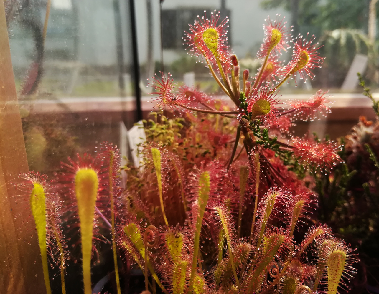
The dataset contains 150 observations of leaf and petiole size for five
varieties of three African sundew species: the typical and red forms of
the Cape sundew, Drosera
capensis, (left), the
typical form of Drosera
madagascarienis
(center) and the typical and anthocyanin-reduced forms of Drosera
venusta (right, photos
taken by myself). 
It is published under a Creative Commons Zero
license, so it
is free to use in any kind of commercial or non-commercial setting. In
particular, if you need a replacement dataset for iris for the
examples in your R package, feel free to add drosera to the package
without any additional precautions.
However, it would be kind if you add a link to the package’s Github page in case you decide to use it (and maybe drop me a line so I can link your project in the repository), but I won’t be mad if you don’t.
Drosera is a wide-spread genus of carnivorous plants (around 200 species) in the family Droseraceae that catch their (mostly insect) prey with a sticky trap mechanism based on a mucilaginous secretion from stalked glands covering their leaf surface. The glistering drops of mucilage on their tentacle-like glands have earned them the common name sundews.
The drosera data package can be installed from Github using
remotes::install_github():
# install remotes package if necessary
install.packages("remotes")
# install corrmorant from the github repository
remotes::install_github("r-link/drosera")
Afterwards, the package can be loaded regularly via library() to
access the data:
library(drosera)
data(package = "drosera")
Afterwards, the drosera data can be used as a regular loaded dataset:
head(drosera)## species variety petiole_length petiole_width blade_length blade_width
## 1 capensis rubra 54.00 1.95 38.30 3.95
## 2 capensis rubra 45.90 1.15 27.60 2.95
## 3 capensis rubra 21.20 0.85 21.85 2.65
## 4 capensis rubra 56.40 1.65 38.20 3.30
## 5 capensis rubra 28.60 1.00 15.80 2.80
## 6 capensis rubra 32.85 1.50 24.65 4.40
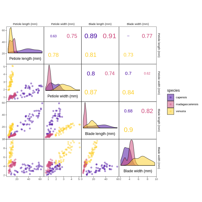
The dataset shows strong correlations between the different variables,
and pronounced inter- and intraspecific differences. Here’s a basic
illustration based on the
corrmorant package.
# load packages
library(tidyverse)
library(corrmorant)

# create plot
ggcorrm(drosera,                                 # dataset
        aes(color = species, fill = species),    # settings of non-standard aesthetics: color and fill by species
        labels = paste(str_to_sentence(gsub("_", " ", names(drosera)[3:6])), "(mm)")) + # labels for variable names
  lotri(geom_point(alpha = 0.4)) +               # points in lower triangle
  utri_corrtext() +                              # indicator of (Pearson) correlation in upper triangle
  dia_density(color = "black", size = .3, alpha = .5) + # density plots on the plot diagonal
  dia_names() +                        # variable names on the plot diagonal
  scale_color_viridis_d(option = "C", begin = .1, end = .9,  # color scale settings
                        aesthetics = c("fill", "color"))
## The following column names were replaced:
## petiole_length -> Petiole length (mm)
## petiole_width -> Petiole width (mm)
## blade_length -> Blade length (mm)
## blade_width -> Blade width (mm)
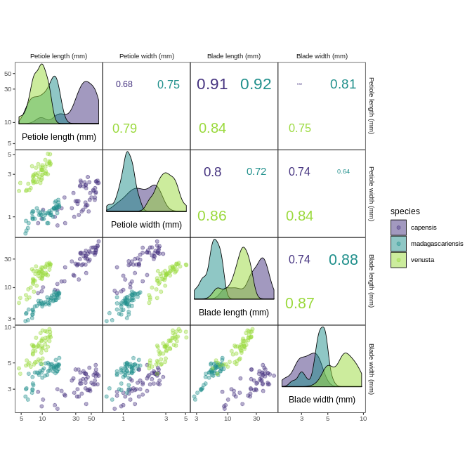
The patterns become even clearer when assessed on a log scale:
ggcorrm(
  drosera,
  aes(color = species, fill = species),
  labels = paste(str_to_sentence(gsub("_", " ", names(drosera)[3:6])), "(mm)")) +
  lotri(geom_point(alpha = 0.4)) +
  utri_corrtext() +
  dia_density(color = "black", size = .3, alpha = .5) +
  dia_names() +
  scale_color_viridis_d(begin = .15, end = .85, aesthetics = c("fill", "color")) +
  scale_x_log10() + scale_y_log10()
## The following column names were replaced:
## petiole_length -> Petiole length (mm)
## petiole_width -> Petiole width (mm)
## blade_length -> Blade length (mm)
## blade_width -> Blade width (mm)
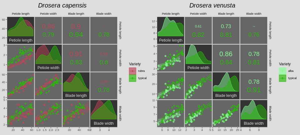
Notably, for the two species where different varieties were measured, there are also subtle but notable differences between the distinct forms:
# Function for plots
pfun <- function(data){
  ggcorrm( data,
    aes(color = variety, fill = variety),
    bg_dia   = "grey20",
    bg_lotri = "grey40",
    bg_utri  = "grey40",
    labels = paste(str_to_sentence(gsub("_", " ", names(drosera)[3:6]))),
  ) +
    lotri(geom_smooth(alpha = .3, method = "lm", size = .35)) +
    lotri(geom_point(alpha = .65)) +
    utri_corrtext(ncol = 1, squeeze = .3) +
    dia_density(alpha = .5) +
    dia_names(col = "#DDDDDD") +
    theme(panel.border    = element_rect(fill = NA, color = "#DDDDDD", size = .8),
          legend.background = element_blank(),
          plot.background = element_rect(fill = "#DDDDDD", , color = "#DDDDDD"),
          plot.title = element_text(face = "italic", hjust = 0.5, size = 15))
}

# Create plot for Drosera capensis
capensis <- pfun(filter(drosera, species == "capensis")) +
    scale_color_manual(values = c("#BB4456", "#25BB04"), aesthetics = c("color", "fill"),
                       name = "Variety") +
    ggtitle("Drosera capensis")

# Create plot for Drosera venusta
venusta <- pfun(filter(drosera, species == "venusta")) +
  scale_color_manual(values = c("#88FF96", "#25BB04"), aesthetics = c("color", "fill"),
                     name = "Variety") +
  ggtitle("Drosera venusta")

# Combine both plots using cowplot::plotgrid()
cowplot::plot_grid(capensis, venusta, nrow = 1) +
  theme(plot.background = element_rect(fill = "#DDDDDD", color = NA))
You can clearly see that for Drosera capensis, the plants of the red form have notably more slender leaves and petioles than the typical form. For Drosera venusta, the differences in proportions were less pronounced, but the plants of the anthocyanin-reduced form on average are smaller than the plants of the typical plants.


