The Flow Analysis Summary Statistics Tool for R (fasstr) is a set of R functions to summarize, analyze, trend, and visualize streamflow data. This package summarizes continuous daily mean streamflow data into various daily, monthly, annual, and long-term statistics, completes annual trends and frequency analyses, and provides output tables and plots.
Useful features of this package include the utilization of the tidyhydat package to extract Water Survey of Canada historical streamflow data from a locally saved HYDAT database for analyses, the filtering of years included in analyses (start and end years, excluded years), option to choose water years for analyses instead of calendar years, streamflow data preparation functions, options to save/write plots directly to your computer within the functions, and customizing how missing dates are handled.
To install the fasstr package, you need to install the devtools package then the fasstr package
install.packages("devtools")
devtools::install_github("bcgov/fasstr")
Then to call the fasstr functions you can either load the package using the library() function or access a specific function using a double-colon (e.g. fasstr::calc_daily_stats()). Several other packages will be installed in addition to this package including zyp for trending, ggplot2 for creating plots, and dplyr and tidyr for various data wrangling and summarizing functions, amongst others.
library(fasstr)To use the HYDAT arguments of the fasstr functions, you will need to download the tidyhydat package and a HYDAT database. Installation instructions for both can be found here.
All functions in fasstr require a record of daily mean streamflow from a hydrometric station. Long-term and continuous datasets are preferred for most analyses, but seasonal and partial data can be used.
Flow data can be provided to the functions through either the HYDAT or flowdata arguments. When using the HYDAT argument, a Water Survey of Canada station number is required (e.g. HYDAT="08NM116") and its corresponding historical daily streamflow record is extracted from HYDAT using tidyhydat. Installation of both tidyhydat and a HYDAT database is required to use this argument.
Data can alternatively be provided using the flowdata argument as a dataframe with columns of 'Date' (YYYY-MM-DD in date format) and 'Value' (mean daily discharge in cubic metres per second in numeric format). The dataframe can have other columns with other names as the functions will looks for 'Date' and 'Value'. The fasstr functions will not recognize your dates and flow data if the columns are not appropriately named 'Date' and 'Value'. The following is an example of an appropriate flowdata dataframe:
str(flowdata)
#> Classes 'tbl_df', 'tbl' and 'data.frame':    16102 obs. of  2 variables:
#>  $ Date : Date, format: "1972-12-01" "1972-12-02" ...
#> $ Value: num 3 0.94 0.385 0.241 0.207 ...To customize your analyses for specific time periods, you can designate the start and end years of your analysis using the start_year and end_year arguments and remove any unwanted years (for partial datasets for example) by listing them in the excluded_years argument (e.g. excluded_years=c(1990,1992:1994)). Leaving these arguments blank will result in the summary/analysis of all years of the provided dataset.
To group analyses by water, or hydrologic, years instead of calendar years, if desired, you can use water_year=TRUE within most functions (default is water_year=FALSE). A water year can be defined as a 12-month period that comprises a complete hydrologic cycle (wet seasons can typically cross calendar year), typically starting with the month with minimum flows (the start of a new water recharge cycle). As water years commonly start in October, the default water year is October for fasstr. If another start month is desired, you can choose is using the water_year_start argument (numeric month) to designate the water year time period. The water year label is designated by the year it ends in (e.g. water year 2000 goes from Oct 1, 1999 to Sep 30, 2000). Start, end and excluded years will be based on the specified water year.
For annual yield runoff statistics calculated in the annual statistics functions, an upstream drainage basin area (in sq. km) is required with the basin_area argument. If no area is supplied with flowdata all yield results will be NA. If using the HYDAT argument to supply streamflow data, the function will automatically use the basin area of the station provided in HYDAT, if available, so basin_area is not required. To override the basin area from HYDAT, set the basin_area to your choosing and it will replace the HYDAT number.
If not using HYDAT and your flowdata dataframe contains a column called STATION_NUMBER (HYDAT originated) the functions will look up the station number listed and grab the corresponding basin area from HYDAT, if it exists, without setting the basin_area argument. This allows you to use a flowdata dataframe that originated from HYDAT without having to look up a basin area.
Coming soon.
In most functions that compute statistics or create plots, there is an option to directly write or save the tables and plots to your computer without additional functions. The default directory is your working directory, but you can choose your directory using the report_dir argument. Tables are saved in '.csv' format and plots can be saved several formats (including '.pdf','.png','.jpeg','.tiff', or '.bmp'), with the default being '.pdf'.
To determine the summary statistics of an entire dataset and by month (mean, median, maximum, minimum, and some percentiles) you can use the calc_longterm_stats() function. If the 'Mission Creek near East Kelowna' hydrometric station is of interest you can list the station number in the HYDAT argument to obtain the data (if tidyhydat and HYDAT are installed).
calc_longterm_stats(HYDAT = "08NM116")
#>        Month      Mean Median Maximum Minimum    P10    P90
#> 1        Jan  1.085907  0.878    9.50   0.160 0.5200  1.700
#> 2        Feb  1.043398  0.879    4.41   0.140 0.4970  1.775
#> 3        Mar  1.606463  1.180    9.86   0.380 0.7050  3.246
#> 4        Apr  6.702245  4.250   42.40   0.340 1.1700 15.600
#> 5        May 23.419247 21.200   87.50   0.821 8.8720 40.200
#> 6        Jun 22.436086 20.300   86.20   0.450 6.2000 40.800
#> 7        Jul  5.981690  3.720   76.80   0.332 0.9946 13.300
#> 8        Aug  2.082254  1.480   22.40   0.311 0.6990  4.022
#> 9        Sep  2.415459  1.560   18.30   0.354 0.6908  5.010
#> 10       Oct  2.121410  1.650   15.20   0.025 0.7797  4.130
#> 11       Nov  1.841419  1.560   11.70   0.260 0.5987  3.291
#> 12       Dec  1.248250  1.080    7.30   0.342 0.5288  2.210
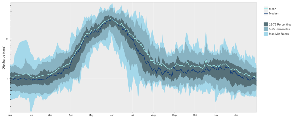
#> 13 Long-term 6.553322 1.840 87.50 0.025 0.6930 21.000To visualize the daily streamflow patterns on an annual basis, the plot_daily_stats() function will plot out various summary statistics for each day of the year. Data can also be filtered for certain years of interest (a 1981-2010 normals period for this example) using the start_year and end_year arguments. Multiple plots are produced with this function, so this example plots just the summary statistics ([1]).
plot_daily_stats(HYDAT = "08NM116",
                 start_year = 1981,
                 end_year = 2010,
                 log_discharge = TRUE)[1]
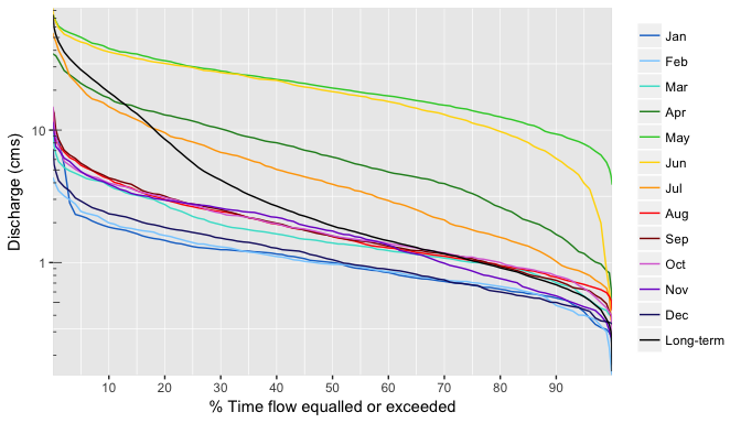
#> $daily_statisiticsFlow duration curves can be produced using the plot_flow_duration() function.
plot_flow_duration(HYDAT = "08NM116",
                   start_year = 1981,
end_year = 2010)This package also provides a function, compute_frequency_analysis(), to complete frequency analyses (using the same methods as HEC-SSP). The default fitting distribution is 'log-Pearson Type III', but the 'weibull' distribution can also be used. Other default plotting and fitting methods are described in the function documentation. For this example, the 7-day low-flow (low-flow is default) quantiles are calculated for the Mission Creek hydrometric station using the 'log-Pearson Type III' distribution. With this, several low-flow indicators can be determined (i.e. 7Q5, 7Q10).
compute_frequency_analysis(HYDAT = "08NM116",
                           start_year = 1981,
                           end_year = 2010,
                           rolling_days=7)[5]
#> $fitted_quantiles
#>    Distribution Probability Return Period Q007-day-Avg
#> 1          PIII       0.010    100.000000    0.1929445
#> 2          PIII       0.050     20.000000    0.2770067
#> 3          PIII       0.100     10.000000    0.3318582
#> 4          PIII       0.200      5.000000    0.4084737
#> 5          PIII       0.500      2.000000    0.5881156
#> 6          PIII       0.800      1.250000    0.8122160
#> 7          PIII       0.900      1.111111    0.9463443
#> 8          PIII       0.950      1.052632    1.0651498
#> 9          PIII       0.975      1.025641    1.1735280
#> 10         PIII       0.980      1.020408    1.2066583
#> 11 PIII 0.990 1.010101 1.3050198This package is under development. This package is maintained by the Water Protection and Sustainability Branch of the British Columbia Ministry of Environment and Climate Change Strategy.
To report bugs/issues/feature requests, please file an issue.
If you would like to contribute to the package, please see our CONTRIBUTING guidelines.
Please note that this project is released with a Contributor Code of Conduct. By participating in this project you agree to abide by its terms.
Copyright 2017 Province of British Columbia

Licensed under the Apache License, Version 2.0 (the "License");
you may not use this file except in compliance with the License.
You may obtain a copy of the License at

   http://www.apache.org/licenses/LICENSE-2.0

Unless required by applicable law or agreed to in writing, software
distributed under the License is distributed on an "AS IS" BASIS,
WITHOUT WARRANTIES OR CONDITIONS OF ANY KIND, either express or implied.
See the License for the specific language governing permissions and
limitations under the License.


