LBM Simulator - Cylindrical Moving Boundary

This project aims to simulate multiple cylindrical moving objects in an unified flow. The fluid behavior and the interaction between cylindrical solid object are described by Lattice-Boltzmann Method (LBM) and modified bouncing-back rule. The programs are written in C and OpenCL for CPU/GPU offloading support, with improved processing speed and memory management.

Before you start using this simulator, take a look at this note: What's the physics of this LBM simulation?.

A high resolution simulation result of above 3 cylinders example:

Video: 3cir_1080p.mp4
Device: NVIDIA GeForce GTX 660
Resolution: 1920x1080 pixels.
Compute time: 5637.89 seconds for 10000 iterations.

Build from Source
Quick Start
Start a Simulation Step by Step
Design and Analyze an Experiment
Troubleshooting

Build from Source

Dependences

Most C programs are written in ISO C. However some of the environmental configuration would be nasty for clang when you are compiling OpenCL kernel program. glibc is recommended instead. As for the The OpenCL driver, it really depends on the platform you have. You should check your OS instruction for the driver packages needed. In Archlinux they are

Runtime

OpenCL (For C binary)
- Intel GPU: intel-compute-runtime
- Intel CPU: intel-opencl-runtime<sup>AUR</sup>
- Nvidia GPU: opencl-nvidia
- AMD GPU: opencl-mesa
- AMD CPU: Not supported anymore.
Tools (For shell script)
- time: Linux built-in, GNU version also works.
- gnuplot: For data analysis and visualization.
- ffmpeg: For MP4 video generation.
- clinfo: good for monitoring all possible platform properties of the system.

Development

ICD loader: ocl-icd
Headers: opencl-headers

Be advice that the Opencl target version need to be defined in you host program as #define CL_TARGET_OPENCL_VERSION 300. while 300 stands for the version 3.0.0. Additionally, C11 Atomic operations support for 64-bits integer is required by the force calculation in simulate_ocl.cl, you will need to check if the device extension of cl_khr_int64_atomics is available for your desire platform.

Build processes

The programs can be built and installed with:

$> cd LBM_CYMB/src
$> make
$> make install

make install will copy all binaries and OpenCL kernel source file into LBM_CYMB/bin. Clean all binaries with make clean if you want a fresh make.

Quick Start

Inside the directory there has:

./
├── bin
├── exp_sets
├── img
├── physics.md
├── README.bak
├── README.md
├── schedule
├── simulator
├── speed_test
└── src

4 directories, 6 files

Three Bash wrapper scripts are written for different procedures:

Simulator

To start an example simulation:

$ ./simulator exp_sets/example
[Parameters]: (* config value)
	<Stratage>
		1. Similarity for the Reynolds number
		2. Spectify CL for CT
	<Dimensionless>
	 *	Mach number(MA): 0.300000
		Reynolds number: 236.514634
		Grid Reynolds number: 0.131397
	<Lattice unit>
	 *	Collision frequency(CF): 0.550000
		Kinematic viscosity: 1.318182
	 *	BCV D: 0.300000 Ux: 0.100000 Uy: 0.000000
	 *	Size nx: 800 ny: 600
		Speed of sound(Csl): 0.333333
	<Conversion factors>
	 *	Length(CL): 1.000000 (m/lattice space)
		Time(CT): 0.001698 (secs/time step)
	 *	Density(CD): 1.225000kg/m^3
		Mass: 1.225000kg
		Force: 1274490.000000kg*m/s^2
		Spring constant: 1274490.000000kg/s^2
		Damping constant: 1249.500000kg/s
	<SI unit>
		Kinematic viscosity: 448.181818m^2/s
		Size width: 800.000000m height: 600.000000m
	 *	Speed of sound(CS): 340.000000m/s
		BCV D: 0.367500kg/m^3 Ux: 102.000000m/s Uy: 0.000000m/s
	<Dirty tricks>
	 *	REFUEL_RTO: 0.500000
	 *	EAT_RTO: 0.050000
	<Objects>
		[spring] [damping] [mass] [Nau_freq] [Nau_cyc]
		0: 127449.000000kg/s^2 12495.000000kg/s 1225.000000kg 1.623380Hz 0.615999s
		1: 127449.000000kg/s^2 12495.000000kg/s 1225.000000kg 1.623380Hz 0.615999s
		2: 127449.000000kg/s^2 12495.000000kg/s 1225.000000kg 1.623380Hz 0.615999s
Simulate......3/100

example directory collect the environmental setups for the simulation. Visulaized data will be generated in example/output with MP4 format, while the kinetic parameters like speeds and accelerations of the cylinders will be recorded in data.

File	Describe
output/0.mp4	Density matrix
output/1.mp4	Speed matrix in x axis
output/2.mp4	Speed matrix in y axis
data	Kinetics data of cylinders

If anything happen unexpected, please refer to Troubleshooting.

schedule

If multiple simulations need to be performed, write a list 3c.sch like this

$ cat 3c.sch
exp_sets/3c_480p
exp_sets/3c_720p
exp_sets/3c_1080p

and the sequence can be initiated with:

$ ./schedule 3c.sch

speed_test

Sometime before an experiment, benchmarking is necessary. Choose the experiment setup and all available devices and working group sizes will be tested.

$ ./speed_test ext_sets/example
	...
	...
	...
	2/0/80/60...	N/A
	2/0/40/30...	N/A
	2/0/32/24...	4.17                                              
	2/0/20/15...	4.31                                              
	2/0/16/12...	4.12                                              
	2/0/8/6...	5.10                                              
	2/0/4/3...	9.24                                              
completed!
Results:
0/0/16/12	17.74
0/0/8/6		17.82
0/0/4/3		22.50
2/0/16/12	33.20
2/0/32/24	33.67
2/0/20/15	35.24
2/0/8/6		43.44
2/0/4/3		85.32
1/0/20/15	95.82
1/0/8/6		97.87
1/0/4/3		98.80
1/0/16/12	98.81
1/0/32/24	99.74
1/0/40/30	100.69
1/0/80/60	103.15
1/0/100/75	104.41

N/A means that this setup cannot be adopted by OpenCL driver. According to the test above, following setup will have the best performance:

PLATFORM 0
DEVICE 0
WORK_ITES_0 16
WORK_ITES_1 12

Use clinfo -l to find out what excetly the devices are:

Platform #0: Intel(R) OpenCL HD Graphics
 `-- Device #0: Intel(R) UHD Graphics 620 [0x3ea0]
Platform #1: Intel(R) OpenCL
 `-- Device #0: Intel(R) Core(TM) i7-8565U CPU @ 1.80GHz
Platform #2: NVIDIA CUDA
 `-- Device #0: NVIDIA GeForce MX150

However, be advice that even the experiment setup can be executed, the actual result may not be correct (exceed maximum flow speed in Lattice-Boltzmann assumption for example). please refer to Strange Video Output.

Start a Simulation Step by Step

Following steps can be altered by your own needs, feel free to play around with it.

Choose a Resolution

To decide a good resolution for the simulation, you should consider with:

The fluid phenomenon you are studying at.

The higher the resolution is, the more accurate simulation you get. However there dose not have a good calculation to tell you what resolution is enough for you, the only approach is benchmarking.
The device you are using.

All devices will have their own preferred work-group-size-multiple affected by the number of compute units and the size of cache. Check the value with clinfo. Most of the case, Intel CPU will go for 128 multiple, while GPU will go for 32 multiple. A simple approach is following the screen resolution, since it is how GPU is designed for. However it may not always be the best one for sure.

Make an Experiment Setup

Inside an experiment setup directory we have:

.
├── a.bc
├── a.nd
├── data
├── default.conf
├── log
└── output
    ├── 0.mp4
    ├── 1.mp4
    └── 2.mp4

1 directory, 8 files

To perform an experiment, you will need to tweak these files:

Name	Description
a.bc	Boundary condition file
a.nd	Number Density file
default.conf	Main configuration file

And following files are used to collect and analyze data.

Name	Description
data	Kinetics data for cylinders
log	Running conditions and status
output/	Result videos or ND files

ND (Number Density) file

Number density matrix describe particle densities in different velocities and positions. A D2Q9 ND file, with 480x270 in size, is formatted as

480 270 9
[m0q0] [m0q1] [m0q2] ...
[m1q0] [m1q1] [m1q2] ...
[m2q0] [m2q1] [m2q2] ...
...

Use nd_gen to make an initial ND file with following options:

Usage: nd_gen [OPTION]
Otions:
	-x #, Numer of column
	-y #, Number of row
	-d #, Density (Default: 0.3)
	-i #, Ux (Default: 0.12)
	-j #, Uy (Default: 0)
	-h , Print this help page
Example:
	nd_gen -x 100 -y 30 -d 0.3 -i 0.1 -j 0 > exp_sets/example/a.nd

BC (Boundary Condition) file

Boundary condition include following classes:

BCV: Unified fluid that surround the simulation area.
CY: Cylinder object.

For example:

bc_no 2
bc_nq 2
BCV {
	dnt 1
	ux 0.0
	uy 0.0
}
CY {
	spring 0.1
	damp 0
	mass 1000
	rad 20
	force 0 0
	acc 0 0
	vel 0 0
	dsp 10 0
	pos 250 70
}
CY {
	spring 0.1
	damp 0
	mass 1000
	rad 20
	force 0 0
	acc 0 0
	vel 0 0
	dsp 10 0
	pos 250 150
}

Parameter	Description
bc_no	Number of objects
bc_nq	Kinematic dimension of objects, usually 2 in 2D simulation.
dnt	Density
ux	Macro velocity in x axis
uy	Macro velocity in y axis
spring	Spring constant of the cylinder, in lattice unit
force	Initial value of applied force of the cylinder, in lattice unit
damp	Damping constant of the cylinder, in lattice unit
mass	Mass of the cylinder, in lattice unit
rad	Radius of the cylinder, in lattice unit
force	Initial value of applied force of the cylinder, in lattice unit
acc	Initial value of applied force of the cylinder, in lattice unit
vel	Initial value of velocities of the cylinder, in lattice unit
dsp	Initial value of displacements of the cylinder, in lattice unit
pos	Initial value of positions of the cylinder, in lattice unit

.conf file

Following parameters are included in a configuration file:

Parameter	Description	Default
LOOP	Iteration of `SKP`.	1
SKP	Iteration of fluid propagate by time step.	1
CF	Collision frequency in Lattice unit	1
CS	Speed of sound in SI unit.	340
CL	Dimensional value of length	1
CD	Dimensional value of Density	1
MA	Mach number(Dimensionless)	0.1
IS_MP4	Make mp4 videos or not.	0
IS_SAVE_DATA	Save final ND matrix or not.	0
IS_FILE_OUTPUT	Save ND matrix for every loops or not.	0
ND_FILE	ND filename	NULL
BC_FILE	BC filename	NULL
OUTPUT_DIR	Output filename	NULL
PROGRAM_FILE	OpenCL source filename	NULL
REFUEL_RTO	Refuel ratio	0.8
EAT_RTO	Eat ratio	0.01
LOG_FILE	Log filename	NULL
DATA_FILE	Data filename	NULL
IS_PAR_PRINT	Print log to stdout or not.	1
IS_PROGRESS_PRINT	Print progress or not	1
PL_MAX_D	Maximum density value for the jetcolormap ploting	0.5
PL_MAX_UX	Maximum x velocity value for the jetcolormap ploting	0.1
PL_MAX_UY	Maximum y velocity value for the jetcolormap ploting	0.1
PLATFORM	Working platform for OpenCL	0
DEVICE	Working device for OpenCL	0
WORK_ITEM_0	Work-group size in dimension 0	1
WORK_ITEM_1	Work-group size in dimension 1	1

Platform & Device

A platform is an specific OpenCL implementation, e.g. Intel, AMD or Nvida CUDA. A device is the actual processor that perform the calculation, like Intel(R) Core(TM) i7-8565U CPU @ 1.80GHz, NVIDIA GeForce MX150.
Work-group & Work-item

A work-group is processed by a single compute unit in the device. For a CPU device it prefer a larger work-group size, while a GPU works opposite. The amount of work-item in a work-group has its limitation, check Max work group size for the value (use clinfo). For multi-dimension work-group, the total amount of work-item cannot exceed Max work group size, and the work-item in each dimension will have their own limitation. Check Max work item sizes for the value.

Use the script speed_test to choose the best environment setup. If the chosen work-group size exceeds the max allowed work-group size for the device, the result will not be printed. Example:

Perform an experiment

Run simulator with desire experiment setup:

$> ./simulator exp_sets/1920x1080

If multiple experiments are going to be launched at once, use schedule plus a plain text list file of experiment setups directory name, like:

$> cat exp_grp1
exp_sets/480x270_skp10
exp_sets/480x270_skp20
exp_sets/480x270_skp30
exp_sets/480x270_skp40
exp_sets/480x270_skp50

And launch with:

$> ./schedule exp_grp1

Present the Results

There are 4 types of results generated by program.

DATA_FILE (Recommended)

Usually the file path defined in DATA_FILE is used to collect all kind of text-based data. By default, BC_print will print all kinetic parameters of all objects in the following format:

#[obj][time][force][acc][vel][dsp][pos]
0 0.000000 10946785.783500 0.000000 2958.925152 0.000000 58.211965 0.000000 0.000000 0.00000 0 180.000000 135.000000
1 0.000000 10946785.783500 0.000000 2958.925152 0.000000 58.211965 0.000000 0.000000 0.00000 0 300.000000 135.000000
0 0.019608 8164637.838000 0.000000 2128.069005 0.000000 100.661622 0.000000 1.141411 0.00000 0 181.141411 135.000000
1 0.019608 8164637.838000 0.000000 2128.069005 0.000000 100.661622 0.000000 1.141411 0.00000 0 301.141411 135.000000
...

You can adjust this output with any format you want by changing the BC_print function in lbmcl.c.

IS_MP4 (Recommend)

If you set IS_MP4 to 1 in default.conf, the macroscopic matrix of density, velocities in x and y axis in every loops will be printed as PPM image and stream to ffmpeg with pipeline. Since the resolution of the experiment may be very big (something like 1920x1080), the disk usage will easily exceed 50GB if we save all images. Therefore, we do it in pipeline to minimize the number of saved matrix during the process and compress the output in MP4 format.

The maximum and minimum values for jetcolormaps are defined as:

[Density] min: 0 max: PL_MAX_D
[Ux] min:-1 * PL_MAX_UX max: PL_MAX_UX
[Uy] min:-1 * PL_MAX_UY max: PL_MAX_UY

IS_SAVE_DATA

Sometime we want to inspect a phenomenon where the fluid is in its steady state, and it may cost 20k+ iterations to reach that state. In this situation you can run a simulation to steady state once and saved the final ND matrix as fin.nd, which can be used as initial ND matrix a.nd in future experiments.

IS_FILE_OUTPUT (NOT recommend)

With this option set to 1 the program will saved ND matrix in every iterations. As we mention before the disk usage will be massive, it is really not a good idea unless you are running a small test with a small number of iterations.

Design and Analyze an Experiment

Here I will show you a working example for designing and analyzing an experiment. Let's say, today I am curious about the behaviors of two cylinders listed alongside the flow direction, with different separations between them as shown below:

The value we want to control is the initial separations between two cylinders, and all others will stay the same.

Generate and Run a Series of Experiment Setups

First, I will need to generate all experiment setups. Creating a new directory 2c_offset in exp_sets.

2c_offset/
├── cal_offset
├── mkexp_2c
├── offset
├── offset.c
├── plot_offset.p
└── tmp
    ├── a.bc
    ├── a.nd
    ├── data
    ├── default.conf
    ├── log
    └── output

2 directories, 10 files

While tmp stored the template of the flow condition as usual, cal_offset, mkexp_2c, offset and plot_offset.p will be explained later.

Tweak the parameters in this template to fit the fluid environments, like BCV, LOOP and a.nd, etc. Benchmark with speed_test to select the best platform & device configuration, and check the speed of fluid not exceeding three tenths of speed of sound by inspecting the MP4 videos. Next, change the value we want to control (separation in this example) with macros like C1X and C2X:

$> cat a.bc
bc_no 2
bc_nq 2
BCV {
	dnt 0.3
	ux 0.1
	uy 0.0
}
CY {
	spring 0.15
	damp 1
	mass 3000
	rad 20
	force 0 0
	acc 0 0
	vel 0 0
	dsp 0 0
	pos C1X 135
}
CY {
	spring 0.15
	damp 1
	mass 3000
	rad 20
	force 0 0
	acc 0 0
	vel 0 0
	dsp 0 0
	pos C2X 135
}

And now we can write a small script named mkexp_2c to automatic generate all the experiment setups by replacing the macros we just created:

#! /bin/bash
name="2c_offset"
dir=`pwd`
mid="240"
printf "" > 2c.sch
for i in `seq 40 10 160`;do
	rm -r $dir/$name-$i 2> /dev/null
	cp $dir/tmp -r $dir/$name-$i
	sed -i "s/C1X/$((mid-i))/" $dir/$name-$i/a.bc
	sed -i "s/C2X/$((mid+i))/" $dir/$name-$i/a.bc
	printf "create exp_sets/$name-$i\n"
	printf "$dir/$name-$i\n" >> 2c.sch
done

This script will also generate a schedule file named 2c.sch, therefore you can start all of the simulations easily with:

./schedule 2c.sch

Inspect the results

By default, all of the kinetic data are saved in debug in each setups directory. Write a small script named cal_offset to collect all of them with the desire column and generate a plot script plot_offfset.p for Gnuplot as

#! /bin/bash

col="9"
pl="plot_offset.p"
echo "#! /usr/bin/gnuplot" > $pl
chmod a+x $pl
echo "set grid" >> $pl
echo "plot \\" >> $pl
ls | grep 2c_offset- | while read dir;do
	offset=`echo $dir | sed 's/2c_offset-//'`
	cut -f $col -d ' ' $dir/data | tail -n+2 | ./offset > .xoff_$offset
	echo "'.xoff_$offset' w l, \\" >> $pl
done
echo "" >> $pl
echo "pause mouse close" >> $pl

Here I also wrote a small C program offset to calculate the offsets in stream input from debug:

#include<stdio.h>

double a,b;
int main(){
	while(scanf("%lf %lf",&a,&b) > 0){
		printf("%lf\n",b-a);
	}
}

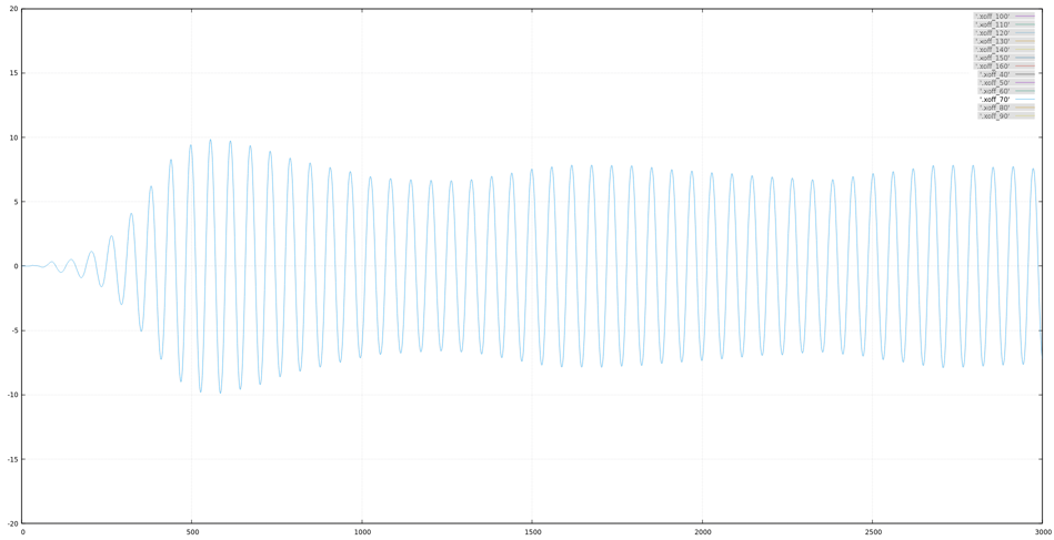
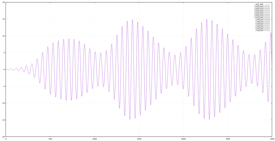
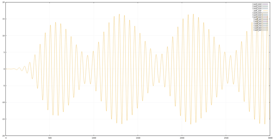
And now we can execute the scripts and generate a chart with the variation of the distance between two cylinders in different initial offsets.

$> cd exp_stes
$> ./cal_offset
$> ./plot_offset.p

The data represent the amount of offset variations between two cylinders in different axis.

X axis

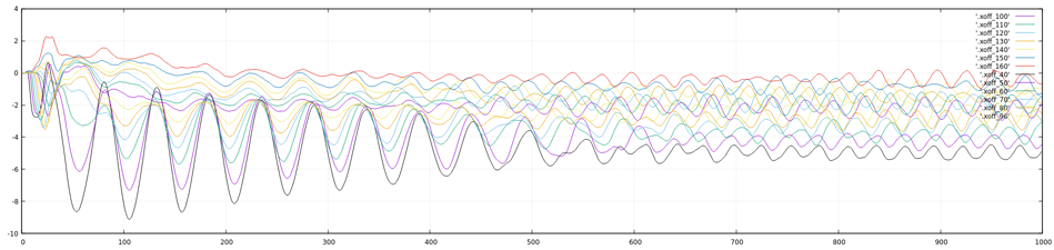Initial separations = 40,60,90,160
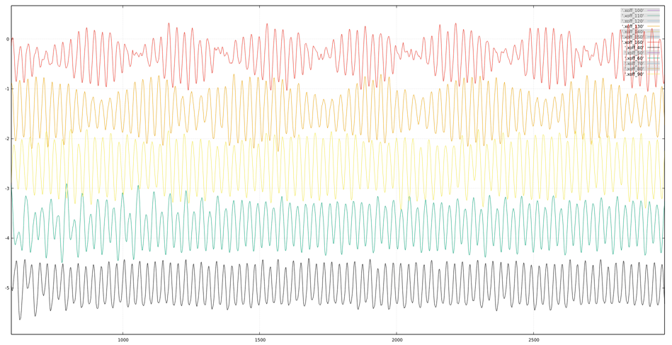
Y axis

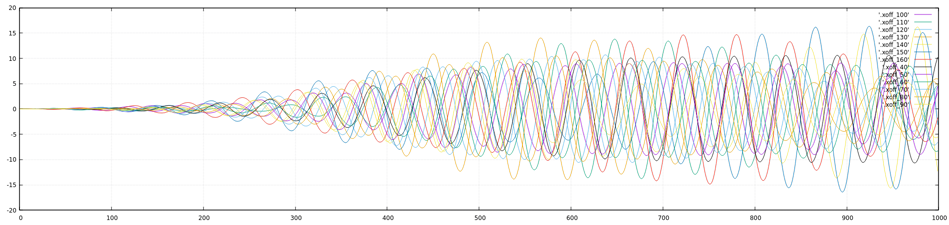separation = 40 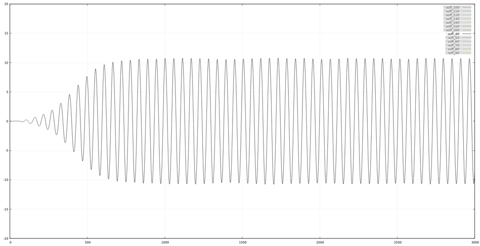separation = 70 separation = 100 separation = 130

Troubleshooting

Before simulation

Platform no exist

If you encounter something like this:

selected platform not exist: p4
real 0.44
user 0.23
sys 0.08

Which means the platform being specifed in ext_sets/example/default.conf didn't exist. Check available platform with clinfo -l, following information should be shown:

Platform #0: Intel(R) OpenCL HD Graphics
 `-- Device #0: Intel(R) UHD Graphics 620 [0x3ea0]
Platform #1: Intel(R) OpenCL
 `-- Device #0: Intel(R) Core(TM) i7-8565U CPU @ 1.80GHz
Platform #2: NVIDIA CUDA
 `-- Device #0: NVIDIA GeForce MX150

If NVIDIA CUDA is the desire one, change the value of PLATFORM to 2 in the configuration file ext_sets/example/default.conf:

..
PLATFORM 2
..

Strange video output

If the video crash on the edge of the cylinder, possible reasons are listed below.

Lake in force variable

Caused by the lake of the GPU memories in each working group. The force acting on the cylinders are collected by long variables between working groups, and the force will be calculated at the end of each loop. Therefore, by reducing the force need to be collected in each loop will solve the problem.

Reduce resolution in a.nd.
Reduce the size of the cylinder in a.bc.
Reduce SKP skip iterations default.conf.
Reduce FC_OFFSET in lbmcl.c and simulate_ocl.cl

Flow/object move too fast

Even the unified flow specified in a.bc may not exceed 1 Mach, the resultant flow speed of the collision might be. Usually happen in high resolution ND matrix, since the lattice flow speed will be larger compared to a lower resolution one. If the object move too fast, the collided flow speed may also exceed the limitation of Lattice-Boltzmann distribution. Following adjustments that slow cylinder down may resolve the problem.

Increase the mass of the cylinder.
Increase the damping ratio of the cylinder.
Reduce the speed of the unified flow.
Increase the collision frequency.

protozis / LBM_CYMB