professorwug / diffusion_curvature_old

Fast, pointwise graph curvature

Diffusion Curvature

Note

The newest code for Diffusion Curvature may be found here. This repository is not maintained, and is preserved only as a monument to the past. There have since been significant enhancements to the diffusion curvature algorithm.

Diffusion curvature is a pointwise extension of Ollivier-Ricci curvature, designed specifically for the often messy world of pointcloud data. Its advantages include:

1. Unaffected by density fluctuations in data: it inherits the diffusion operator’s denoising properties.
2. Fast, and scalable to millions of points: it depends only on matrix powering - no optimal transport required.

Install

To install with pip (or better yet, poetry),

pip install diffusion-curvature

or

poetry add diffusion-curvature

Conda releases are pending.

Usage

To compute diffusion curvature, first create a graphtools graph with your data. Graphtools offers extensive support for different kernel types (if creating from a pointcloud), and can also work with graphs in the PyGSP format. We recommend using anistropy=1, and verifying that the supplied knn value encompasses a reasonable portion of the graph.

from diffusion_curvature.datasets import torus
import graphtools
X_torus, torus_gaussian_curvature = torus(n=5000)
G_torus = graphtools.Graph(X_torus, anisotropy=1, knn=30)

Graphtools offers many additional options. For large graphs, you can speed up the powering of the diffusion matrix with landmarking: simply pass n_landmarks=1000 (e.g) when creating the graphtools graph. If you enable landmarking, diffusion-curvature will automatically use it.

Next, instantiate a DiffusionCurvature operator.

from diffusion_curvature.graphtools import DiffusionCurvature
DC = DiffusionCurvature(t=12)

---

source

DiffusionCurvature

 DiffusionCurvature (t:int, distance_type='PHATE', dimest=None,
                     use_entropy:bool=False, **kwargs)

Initialize self. See help(type(self)) for accurate signature.

	Type	Default	Details
t	int		Number of diffusion steps to use when measuring curvature. TODO: Heuristics
distance_type	str	PHATE
dimest	NoneType	None	Dimensionality estimator to use. If None, defaults to KNN with default params
use_entropy	bool	False	If true, uses KL Divergence instead of Wasserstein Distances. Faster, seems empirically as good, but less proven.
kwargs

And, finally, pass your graph through it. The DiffusionCurvature operator will store everything it computes – the powered diffusion matrix, the estimated manifold distances, and the curvatures – as attributes of your graph. To get the curvatures, you can run G.ks.

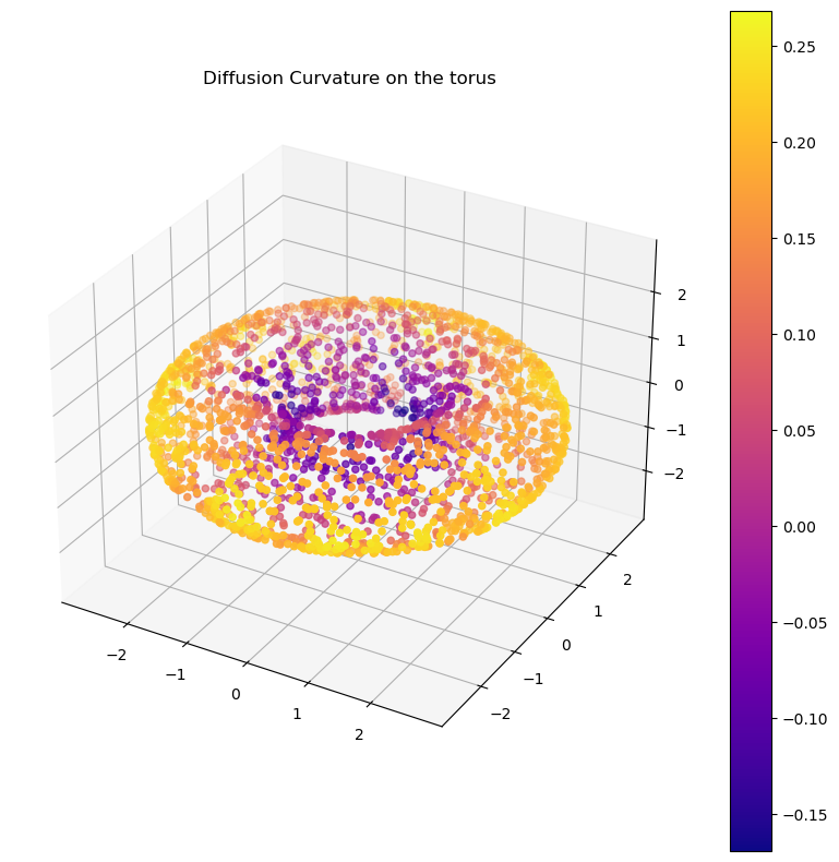
G_torus = DC.curvature(G_torus, dimension=2) # note: this is the intrinsic dimension of the data

plot_3d(X_torus, G_torus.ks, colorbar=True, title="Diffusion Curvature on the torus")

Using on a predefined graph

If you have an adjacency matrix but no pointcloud, diffusion curvature may still be useful. The caveat, currently, is that our intrinsic dimension estimation doesn’t yet support graphs, so you’ll have to compute & provide the dimension yourself – if you want a signed curvature value.

If you’re only comparing relative magnitudes of curvature, you can skip this step.

For predefined graphs, we use our own ManifoldGraph class. You can create one straight from an adjacency matrix:

from diffusion_curvature.manifold_graph import ManifoldGraph, diffusion_curvature, diffusion_entropy_curvature, entropy_of_diffusion, wasserstein_spread_of_diffusion, power_diffusion_matrix, phate_distances
from diffusion_curvature.kernels import gaussian_kernel
import numpy as np

# if you want (or have) to compute your own A
A = gaussian_kernel(X_torus, kernel_type="adaptive", k = 20, anisotropic_density_normalization=1)
np.fill_diagonal(A,0)
# initialize the manifold graph; input your computed dimension along with the adjacency matrix
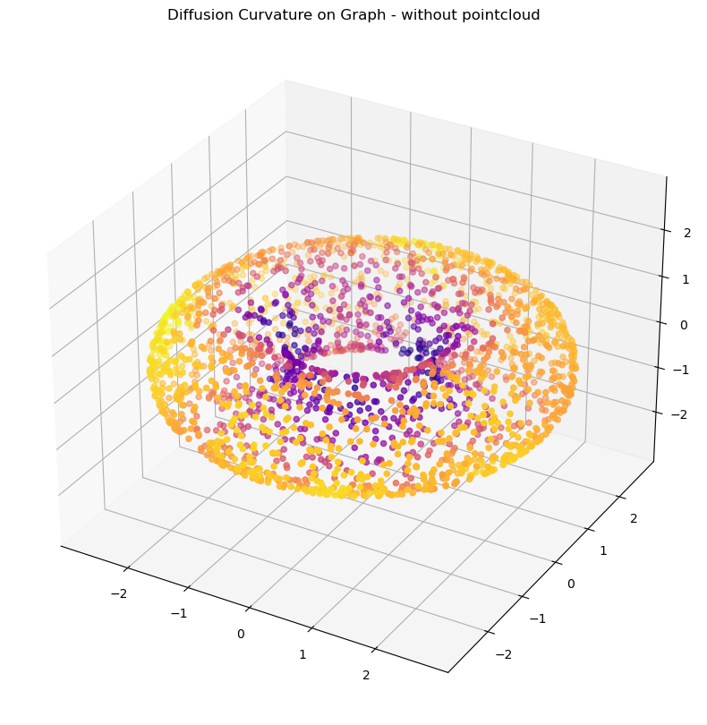
G_pure = ManifoldGraph(A = A, dimension=2, anisotropic_density_normalization=1)

G_pure = diffusion_curvature(G_pure, t=8)
plot_3d(X_torus, G_pure.ks, title = "Diffusion Curvature on Graph - without pointcloud")

Alternately, to compute just the relative magnitudes of the pointwise curvatures (without signs), we can directly use either the wasserstein_spread_of_diffusion (which computes the $W_1$ distance from a dirac to its t-step diffusion), or the entropy_of_diffusion function (which computes the entropy of each t-step diffusion). The latter is nice when the manifold’s geodesic distances are hard to estimate – it corresponds to replacing the wasserstein distance with the KL divergence.

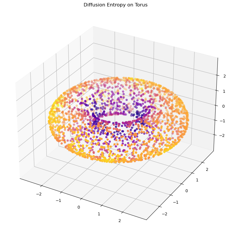
Both of these estimate an “inverse laziness” value that is inversely proportional to curvature. To use magnitude estimations in which the higher the curvature, the higher the value, we can simply take the reciprocal of the output.

# for the wasserstein version, we need manifold distances
G_pure = power_diffusion_matrix(G_pure,t=8)
G_pure = phate_distances(G_pure)
ks_wasserstein = wasserstein_spread_of_diffusion(G_pure)

# for the entropic version, we need only power the diffusion operator
G_pure = power_diffusion_matrix(G_pure, t=8)
ks_entropy = entropy_of_diffusion(G_pure)

plot_3d(X_torus, 1/ks_entropy, title="Diffusion Entropy on Torus")