prakharsharma / CarND-Advanced-Lane-Lines

Advanced Lane Finding Project

The goals / steps of this project are the following:

• Compute the camera calibration matrix and distortion coefficients given a set of chessboard images.
• Apply a distortion correction to raw images.
• Use color transforms, gradients, etc., to create a thresholded binary image.
• Apply a perspective transform to rectify binary image ("birds-eye view").
• Detect lane pixels and fit to find the lane boundary.
• Determine the curvature of the lane and vehicle position with respect to center.
• Warp the detected lane boundaries back onto the original image.
• Output visual display of the lane boundaries and numerical estimation of lane curvature and vehicle position.

Rubric Points

###Here I will consider the rubric points individually and describe how I addressed each point in my implementation.

---

###Writeup / README

####1. Provide a Writeup / README that includes all the rubric points and how you addressed each one. You can submit your writeup as markdown or pdf. Here is a template writeup for this project you can use as a guide and a starting point.

You're reading it! ###Camera Calibration

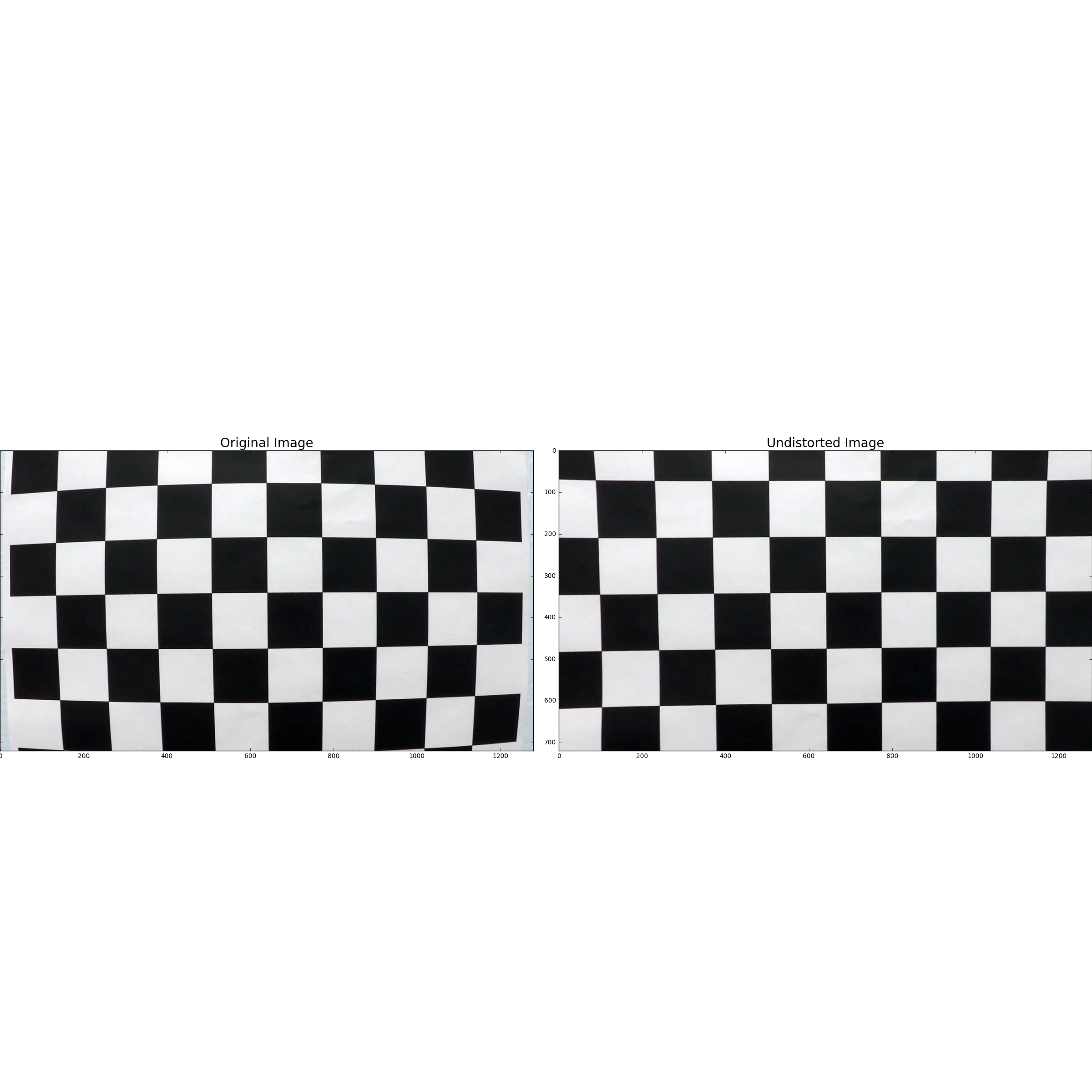
####1. Briefly state how you computed the camera matrix and distortion coefficients. Provide an example of a distortion corrected calibration image.

The code for this step is contained in calibrate of file camera_calibration.py.

I start by preparing "object points", which will be the (x, y, z) coordinates of the chessboard corners in the world. Here I am assuming the chessboard is fixed on the (x, y) plane at z=0, such that the object points are the same for each calibration image. Thus, objp is just a replicated array of coordinates, and objpoints will be appended with a copy of it every time I successfully detect all chessboard corners in a test image. imgpoints will be appended with the (x, y) pixel position of each of the corners in the image plane with each successful chessboard detection.

I then used the output objpoints and imgpoints to compute the camera calibration and distortion coefficients using the cv2.calibrateCamera() function. I applied this distortion correction to the test image using the cv2.undistort() function and obtained this result:

###Pipeline (single images)

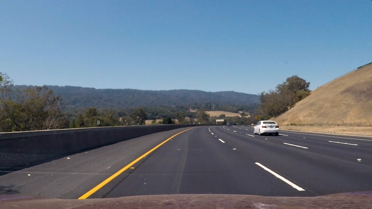
####1. Provide an example of a distortion-corrected image. To demonstrate this step, I will describe how I apply the distortion correction to one of the test images like this one:

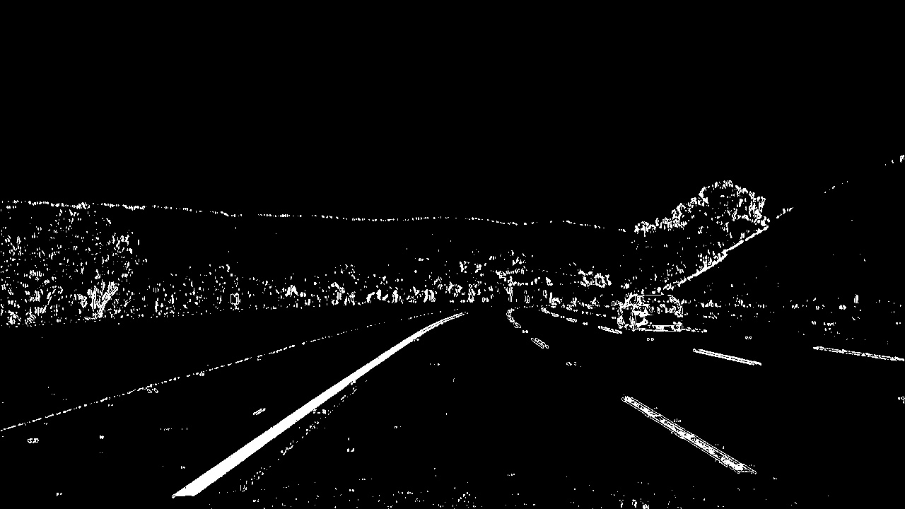
####2. Describe how (and identify where in your code) you used color transforms, gradients or other methods to create a thresholded binary image. Provide an example of a binary image result. I used a combination (logical or) of color (S channel) and gradient (Sobel X) thresholds to generate a binary image. S channel thresholding is done by function sChannel_threshold. Sobel X threshold is done by function binary_threshold. Following values of thresholds were used:

    s_channel_threshold = (170, 255)
    sobel_x_threshold = (20, 100)

Here's an example of my output for this step. (note: this is not actually from one of the test images)

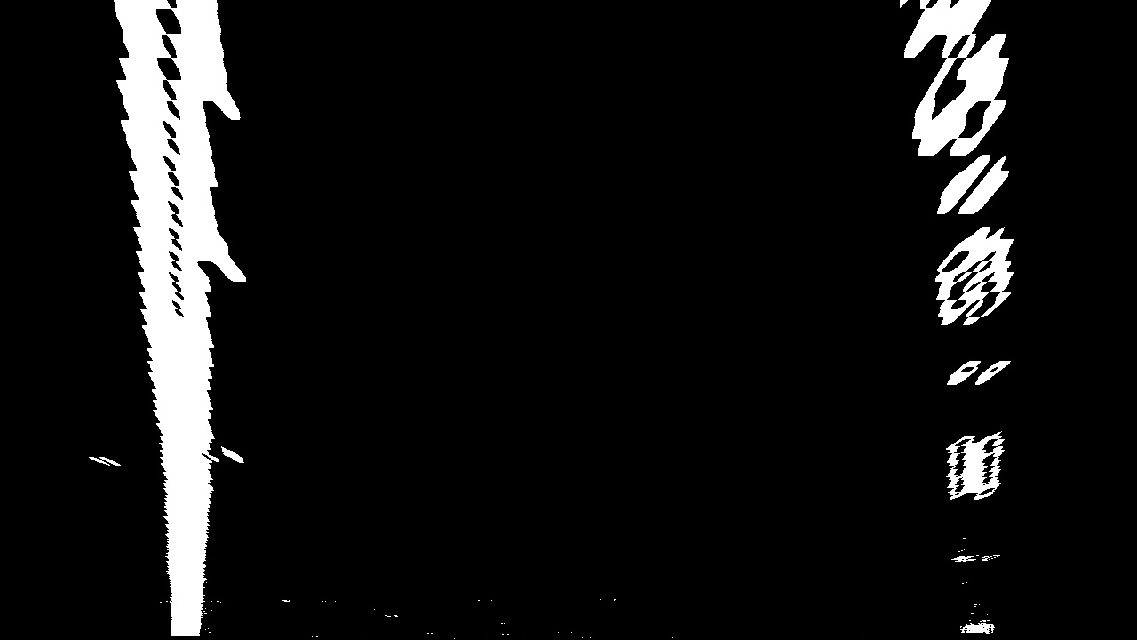
####3. Describe how (and identify where in your code) you performed a perspective transform and provide an example of a transformed image.

Perspective transformation is done by perspective_transform. The function takes as inputs the image to be transformed and does the transformation. It does the transformation using (src) and destination (dst) points which are calculated in the following manner:

    line_len = lambda p1, p2: np.sqrt(
            (p2[0] - p1[0]) ** 2 + (p2[1] - p1[1]) ** 2)

    src = np.float32([
        # top left
        [586., 458.],

        # top right
        [697., 458.],

        # bottom right
        [1089., 718.],

        # bottom left
        [207., 718.]
    ])

    length_of_right_edge = line_len(src[1], src[2])

    rect_width = src[2][0] - src[3][0]
    top_right = [src[2][0], src[2][1] - length_of_right_edge]

    dst = np.float32([
        # top left
        [top_right[0] - rect_width, top_right[1]],

        # top right
        top_right,

        # bottom right
        src[2],

        # bottom left
        src[3]
    ])

I verified that my perspective transform was working as expected by drawing the src and dst points onto a test image and its warped counterpart to verify that the lines appear parallel in the warped image.

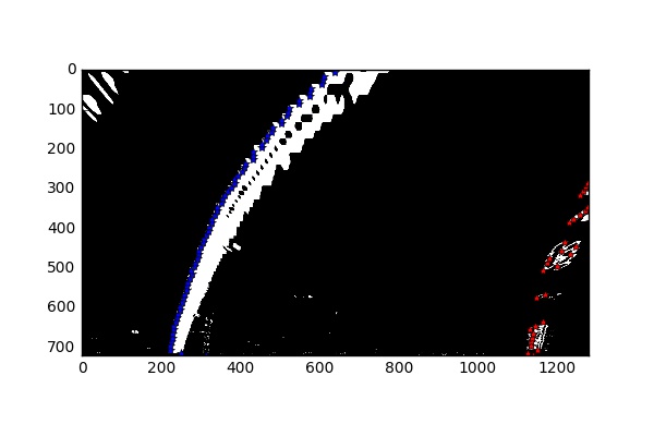
####4. Describe how (and identify where in your code) you identified lane-line pixels and fit their positions with a polynomial?

detect_lane_lines detects lane line pixels and fits a second order polynomial through the detected points.

Starting points of the lane lines are detected as follows

    h, w = image.shape[:2]
    
    histogram = np.sum(warped[h/2:, :], axis=0)
    
    # starting point of left lane, look in left half of the image
    p1 = np.argmax(histogram[:w/2])
    
    # starting point of right lane, look in right half of the image
    p2 = np.argmax(histogram[w/2:])

Using the above starting points, we run a sliding window algorithm up the image to detect pixels for the lane lines. This algorithm is implemented from line#193 to line#257 of function detect_lane_lines.

After detecting lane lines pixels, detect_lane_lines, fits a second order polynomial through them, which look like:

####5. Describe how (and identify where in your code) you calculated the radius of curvature of the lane and the position of the vehicle with respect to center.

Radius of curvature is calculated using the material presented in lecture notes (lecture#34). This is implemented by lane_curvature.

To determine vehicle positon wrt lane center, we use following data points: -

1. Vehicle position wrt to the image (assume vehicle's center to be located at the center of the image).
2. X coordinates of the left and right lane line as per the fitted polynomial at the bottom of the image, i.e., Y = image.shape[0].

This is implemented by vehicle_pos_wrt_lane_center.

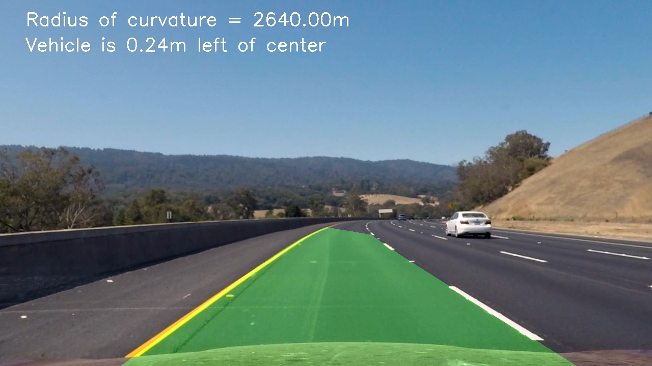
####6. Provide an example image of your result plotted back down onto the road such that the lane area is identified clearly.

Function warp_back draws detected lane lines on the undistorted image and annotates it with calculations for radius of curvature and vehicle position wrt lane center. Here is an example of my result on a test image:

---

###Pipeline (video)

####1. Provide a link to your final video output. Your pipeline should perform reasonably well on the entire project video (wobbly lines are ok but no catastrophic failures that would cause the car to drive off the road!).

Here's a link to my video result

---

###Discussion

####1. Briefly discuss any problems / issues you faced in your implementation of this project. Where will your pipeline likely fail? What could you do to make it more robust?

Problems/issues

I found this project particularly challenging. Main problems for me arose from the following areas

• Lack of familiarity with
  • Material, i.e., computer vision techniques. I had to watch the videos at least twice.
  • Tools - numpy, opencv, ...
• Project required too much time, i.e., too many things to do

Given that it was so challenging, I am pretty proud of what I have put together! Nonetheless, there are quite a few areas of improvement so that its performance can improve say wrt challenge videos.

Areas of improvement

1. Images
   1. Experiment with more ways to form thresholded binary image and different thresholds. May be learn, the best thresholds?
   2. Automatic detection of src and dst points for perspective transform.
   3. Sliding window procedure to detect lane lines uses a configurable window size (100). It will be worthwhile to experiment with different window sizes or may be learn the right window size for an image.
2. Video
   1. Try out ways of smoothing measurements across previous frames other than simple mean.
   2. Build a numerical (between 0 and 1) measure of confidence for detection and use it to qualify detection as good or bad. Some ideas to consider
      1. Width of lane matches to the known lane width (or range of allowed lane widths in the country).
      2. Low variance of lane width in a frame, i.e., detected left and right lines stay parallel to each other.
      3. Low variance of lane width measured across successive frames.
      4. Low variance of radius of curvature measures across frames.
   3. Current implementation looks for lane lines in a window size of 100 (configurable) around the lane line points detected for the previous frame. It is worthwhile to experiment with different window sizes and maybe learn the right window size.
3. Finally, I will like to use deep learning for lane lines detection and compare how it performs against a CV approach.