DiffEqFlux.jl

DiffEqFlux.jl fuses the world of differential equations with machine learning by helping users put diffeq solvers into neural networks. This package utilizes DifferentialEquations.jl and Flux.jl as its building blocks.

Example Usage

For an overview of what this package is for, see this blog post.

Optimizing parameters of an ODE

First let's create a Lotka-Volterra ODE using DifferentialEquations.jl. For more details, see the DifferentialEquations.jl documentation

using DifferentialEquations
function lotka_volterra(du,u,p,t)
  x, y = u
  α, β, δ, γ = p
  du[1] = dx = α*x - β*x*y
  du[2] = dy = -δ*y + γ*x*y
end
u0 = [1.0,1.0]
tspan = (0.0,10.0)
p = [1.5,1.0,3.0,1.0]
prob = ODEProblem(lotka_volterra,u0,tspan,p)
sol = solve(prob,Tsit5())
using Plots
plot(sol)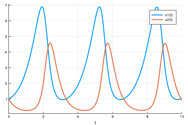

Next we define a single layer neural network that uses the diffeq_rd layer function that takes the parameters and returns the solution of the x(t) variable. Instead of being a function of the parameters, we will wrap our parameters in param to be tracked by Flux:

using Flux, DiffEqFlux
p = param([2.2, 1.0, 2.0, 0.4]) # Initial Parameter Vector
params = Flux.Params([p])

function predict_rd() # Our 1-layer neural network
  Array(diffeq_rd(p,prob,Tsit5(),saveat=0.1))
end

Next we choose a loss function. Our goal will be to find parameter that make the Lotka-Volterra solution constant x(t)=1, so we defined our loss as the squared distance from 1:

loss_rd() = sum(abs2,x-1 for x in predict_rd())

Lastly, we train the neural network using Flux to arrive at parameters which optimize for our goal:

data = Iterators.repeated((), 100)
opt = ADAM(0.1)
cb = function () #callback function to observe training
  display(loss_rd())
  # using `remake` to re-create our `prob` with current parameters `p`
  display(plot(solve(remake(prob,p=Flux.data(p)),Tsit5(),saveat=0.1),ylim=(0,6)))
end

# Display the ODE with the initial parameter values.
cb()

Flux.train!(loss_rd, params, data, opt, cb = cb)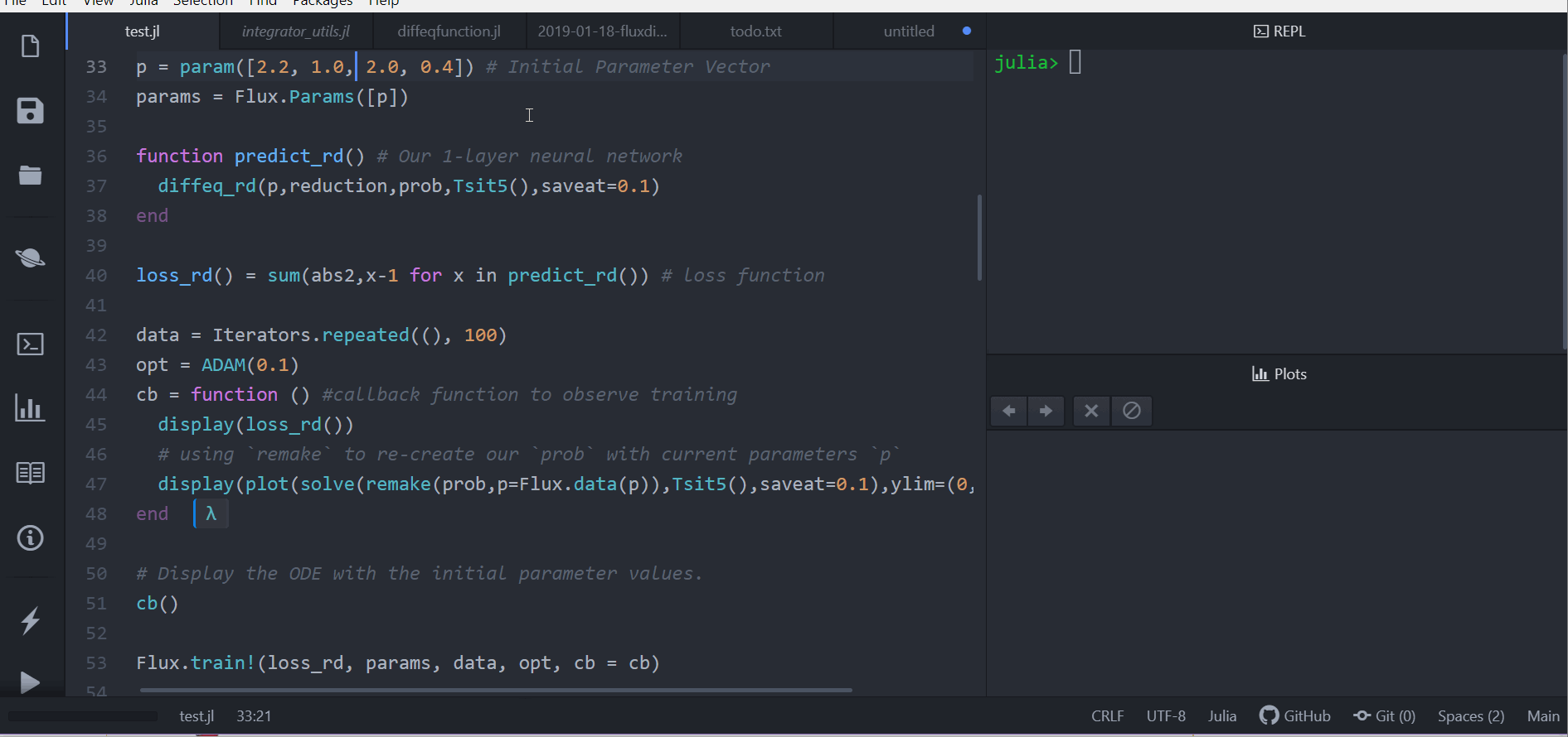

Note that by using anonymous functions, this diffeq_rd can be used as a layer in a neural network Chain, for example like

m = Chain(
  Conv((2,2), 1=>16, relu),
  x -> maxpool(x, (2,2)),
  Conv((2,2), 16=>8, relu),
  x -> maxpool(x, (2,2)),
  x -> reshape(x, :, size(x, 4)),
  # takes in the ODE parameters from the previous layer
  p -> Array(diffeq_rd(p,prob,Tsit5(),saveat=0.1),
  Dense(288, 10), softmax) |> gpu

m = Chain(
  Dense(28^2, 32, relu),
  # takes in the initial condition from the previous layer
  x -> Array(diffeq_rd(p,prob,Tsit5(),saveat=0.1,u0=x))),
  Dense(32, 10),
  softmax)

Using Other Differential Equations

Other differential equation problem types from DifferentialEquations.jl are supported. For example, we can build a layer with a delay differential equation like:

function delay_lotka_volterra(du,u,h,p,t)
  x, y = u
  α, β, δ, γ = p
  du[1] = dx = (α - β*y)*h(p,t-0.1)[1]
  du[2] = dy = (δ*x - γ)*y
end
h(p,t) = ones(eltype(p),2)
prob = DDEProblem(delay_lotka_volterra,[1.0,1.0],h,(0.0,10.0),constant_lags=[0.1])

p = param([2.2, 1.0, 2.0, 0.4])
params = Flux.Params([p])
function predict_rd_dde()
  Array(diffeq_rd(p,prob,MethodOfSteps(Tsit5()),saveat=0.1))
end
loss_rd_dde() = sum(abs2,x-1 for x in predict_rd_dde())
loss_rd_dde()

Or we can use a stochastic differential equation:

function lotka_volterra_noise(du,u,p,t)
  du[1] = 0.1u[1]
  du[2] = 0.1u[2]
end
prob = SDEProblem(lotka_volterra,lotka_volterra_noise,[1.0,1.0],(0.0,10.0))

p = param([2.2, 1.0, 2.0, 0.4])
params = Flux.Params([p])
function predict_fd_sde()
  diffeq_fd(p,reduction,101,prob,SOSRI(),saveat=0.1)
end
loss_fd_sde() = sum(abs2,x-1 for x in predict_fd_sde())
loss_fd_sde()

data = Iterators.repeated((), 100)
opt = ADAM(0.1)
cb = function ()
  display(loss_fd_sde())
  display(plot(solve(remake(prob,p=Flux.data(p)),SOSRI(),saveat=0.1),ylim=(0,6)))
end

# Display the ODE with the current parameter values.
cb()

Flux.train!(loss_fd_sde, params, data, opt, cb = cb)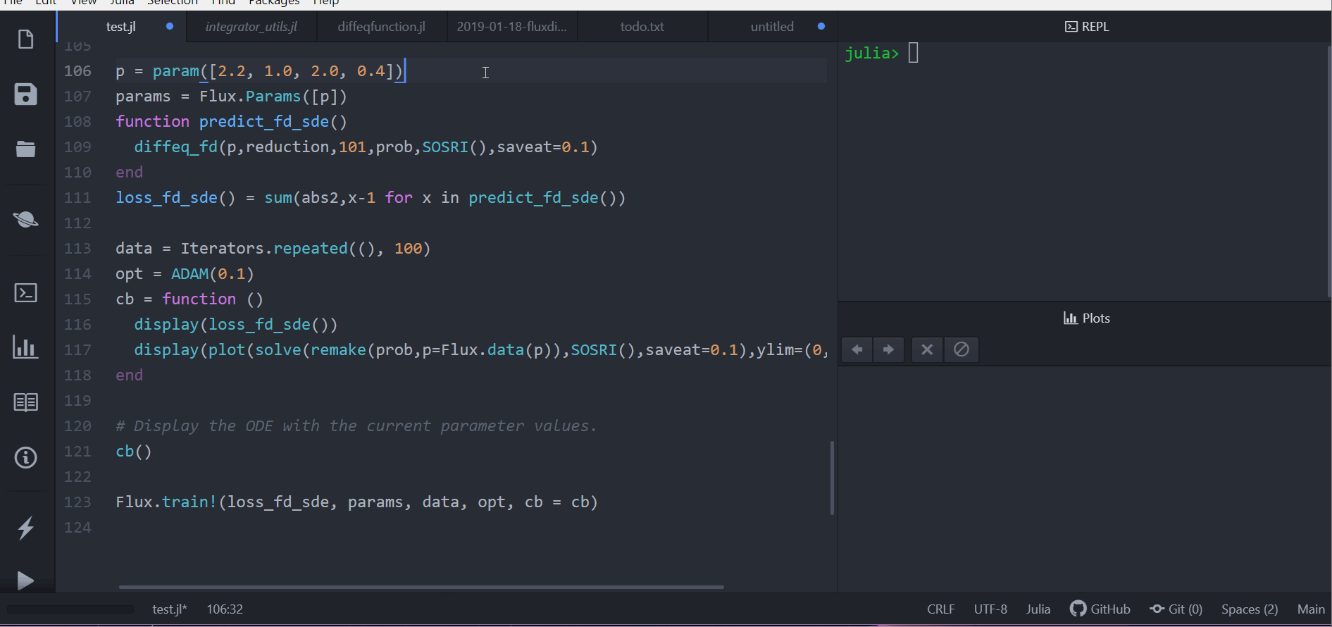

Neural Ordinary Differential Equations

We can use DiffEqFlux.jl to define, solve, and train neural ordinary differential equations. A neural ODE is an ODE where a neural network defines its derivative function. Thus for example, with the multilayer perceptron neural network Chain(Dense(2,50,tanh),Dense(50,2)), a neural ODE would be defined as having the ODE function:

model = Chain(Dense(2,50,tanh),Dense(50,2))
# Define the ODE as the forward pass of the neural network with weights `p`
function dudt(du,u,p,t)
    du .= model(u)
end

A convenience function which handles all of the details is neural_ode. To use neural_ode, you give it the initial condition, the internal neural network model to use, the timespan to solve on, and any ODE solver arguments. For example, this neural ODE would be defined as:

tspan = (0.0f0,25.0f0)
x -> neural_ode(dudt,x,tspan,Tsit5(),saveat=0.1)

where here we made it a layer that takes in the initial condition and spits out an array for the time series saved at every 0.1 time steps.

Training a Neural Ordinary Differential Equation

Let's get a time series array from the Lotka-Volterra equation as data:

u0 = Float32[2.; 0.]
datasize = 30
tspan = (0.0f0,1.5f0)

function trueODEfunc(du,u,p,t)
    true_A = [-0.1 2.0; -2.0 -0.1]
    du .= ((u.^3)'true_A)'
end
t = range(tspan[1],tspan[2],length=datasize)
prob = ODEProblem(trueODEfunc,u0,tspan)
ode_data = Array(solve(prob,Tsit5(),saveat=t))

Now let's define a neural network with a neural_ode layer. First we define the layer:

dudt = Chain(x -> x.^3,
             Dense(2,50,tanh),
             Dense(50,2))
n_ode(x) = neural_ode(dudt,x,tspan,Tsit5(),saveat=t,reltol=1e-7,abstol=1e-9)

And build a neural network around it. We will use the L2 loss of the network's output against the time series data:

function predict_n_ode()
  n_ode(u0)
end
loss_n_ode() = sum(abs2,ode_data .- predict_n_ode())

and then train the neural network to learn the ODE:

data = Iterators.repeated((), 1000)
opt = ADAM(0.1)
cb = function () #callback function to observe training
  display(loss_n_ode())
  # plot current prediction against data
  cur_pred = Flux.data(predict_n_ode())
  pl = scatter(0.0:0.1:10.0,ode_data[1,:],label="data")
  scatter!(pl,0.0:0.1:10.0,cur_pred[1,:],label="prediction")
  plot(pl)
end

# Display the ODE with the initial parameter values.
cb()

Flux.train!(loss_n_ode, params, data, opt, cb = cb)

Use with GPUs

Note that the differential equation solvers will run on the GPU if the initial condition is a GPU array. Thus for example, we can define a neural ODE by hand that runs on the GPU:

u0 = [2.; 0.] |> gpu
dudt = Chain(Dense(2,50,tanh),Dense(50,2)) |> gpu

function ODEfunc(du,u,p,t)
    du .= Flux.data(dudt(u))
end
prob = ODEProblem(ODEfunc, u0,tspan)

# Runs on a GPU
sol = solve(prob,BS3(),saveat=0.1)

and the diffeq layer functions can be used similarly. Or we can directly use the neural ODE layer function, like:

x -> neural_ode(gpu(dudt),gpu(x),tspan,BS3(),saveat=0.1)

API Documentation

DiffEq Layer Functions

diffeq_rd(p,prob, args...;u0 = prob.u0, kwargs...) uses Flux.jl's reverse-mode AD through the differential equation solver with parameters p and initial condition u0. The rest of the arguments are passed to the differential equation solver. The return is the DESolution.
diffeq_fd(p,reduction,n,prob,args...;u0 = prob.u0, kwargs...) uses ForwardDiff.jl's forward-mode AD through the differential equation solver with parameters p and initial condition u0. n is the output size where the return value is reduction(sol). The rest of the arguments are passed to the differential equation solver.
diffeq_adjoint(p,prob,args...;u0 = prob.u0, kwargs...) uses adjoint sensitivity analysis to "backprop the ODE solver" via DiffEqSensitivity.jl. The return is the time series of the solution as an array solved with parameters p and initial condition u0. The rest of the arguments are passed to the differential equation solver or handled by the adjoint sensitivity algorithm (for more details on sensitivity arguments, see the diffeq documentation).

Neural DE Layer Functions

neural_ode(x,model,tspan,args...;kwargs...) defines a neural ODE layer where x is the initial condition, model is a Flux.jl model, tspan is the time span to integrate, and the rest of the arguments are passed to the ODE solver. The parameters should be implicit in the model.
neural_dmsde(x,model,mp,tspan,args...;kwargs) defines a neural multiplicative SDE layer where x is the initial condition, model is a Flux.jl model, tspan is the time span to integrate, and the rest of the arguments are passed to the SDE solver. The noise is assumed to be diagonal multiplicative, i.e. the Wiener term is mp.*u.*dW for some array of noise constants mp.

pochoi / DiffEqFlux.jl