This repository complements the paper Sinkhorn Barycenters with Free Support via Frank-Wolfe Algorithm by Giulia Luise, Saverio Salzo, Massimiliano Pontil and Carlo Ciliberto published at Neural Information Processing Systems (NeurIPS) 2019, by providing an implementation of the proposed algorithm to compute the Barycenter of multiple probability measures with respect to the Sinkhorn Divergence.
Slides can be found here.
If you are interested in using the proposed algorithm in your projects please refer to the instructions here.
Below we provide the code and instructions to reproduce most of the experiments in the paper. We recommend running all experiments on GPU.
- Nested Ellipses
- Barycenter of Continuous Measures(Coming soon)
- Distribution Matching
- k-Means
- Sinkhorn Propagation(Coming soon)
The core dependencies are:
For some experiments we also have the following additional dependencies:
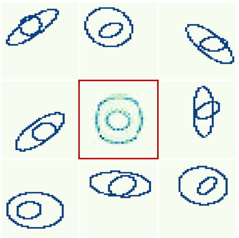
We compute the barycenter of 30 randomly generated nested ellipses on a 50 × 50 pixels image, similarly to (Cuturi and Doucet 2014). We interpret each image as a probability distribution in 2D. The cost matrix is given by the squared Euclidean distances between pixels. The fiture reports 8 samples of the input ellipses (all examples can be found in the folder data/ellipses and the barycenter obtained with the proposed algorithm in the middle. It shows qualitatively that our approach captures key geometric properties of the input measures.

Run:
$ python experiments/ellipses.pyOutput in folder out/ellipses


We compute the barycenter of 5 Gaussian distributions with mean and covariance matrix randomly generated. We apply to empirical measures obtained by sampling n = 500 points from each one. Since the (Wasserstein) barycenter of Gaussian distributions can be estimated accurately (Cuturi and Doucet 2014) (see (Agueh and Carlier 2011)), in the figure we report both the output of the proposed algorithm (as a scatter plot) and the true Wasserstein barycenter (as level sets of its density). We observe that our estimator recovers both the mean and covariance of the target barycenter.
Run:
$ python experiments/gaussians.pyOutput in folder out/gaussians
Instructions for additional experiments and parameters can be found directly in the file experiments/gaussians.py.


Similarly to (Claici et al. 2018), we test the proposed algorithm in the special case where we are computing the “barycenter” of a single measure (rather than multiple ones). While the solution of this problem is the input distribution itself, we can interpret the intermediate iterates the proposed algorithm as compressed version of the original measure. In this sense the iteration number k represents the level of compression since the corresponding barycenter estimate is supported on at most k points. The figure (Right) reports iteration k = 5000 for the proposed algorithm applied to the 140 × 140 image in (Left) interpreted as a probability measure in 2D. We note that the number of points in the support is ∼3900: the most relevant support points are selected multiple times to accumulate the right amount of mass on each of them (darker color = higher weight). This shows that the proposed approach tends to greedily search for the most relevant support points, prioritizing those with higher weight.
Run:
$ python experiments/matching.pyOutput in folder out/matching
The code can be run with any image by passing the path to the desired image as additional argument.

We test the proposed algorithm on a k-means clustering experiment. We consider a subset of 500 random images from the MNIST dataset. Each image is suitably normalized to be interpreted as a probability distribution on the grid of 28 × 28 pixels with values scaled between 0 and 1. We initialize 20 centroids according to the k-means++ strategy. The figure deipcts the corresponding 20 centroids obtained throughout this process. We see that the structure of the digits is successfully detected, recovering also minor details (e.g. note the difference between the 2 centroids).
Run:
$ python experiments/kmeans.pyOutput in folder out/kmeans


We consider the problem of Sinkhorn propagation similar to the Wasserstein propagation in (Solomon et al. 2014). The goal is to predict the distribution of missing measurements for weather stations in the state of Texas, US (data from National Climatic Weather Data) by propagating measurements from neighboring stations in the network. The problem can be formulated as minimizing the functional

over the set 


Run:
$ python experiments/propagation.pyOutput in folder out/propagation
- (this work) G. Luise, S. Salzo, M. Pontil, C. Ciliberto. Sinkhorn Barycenters with Free Support via Frank-Wolfe Algorithm Neural Information Processing Systems (NeurIPS), 2019.
- J. Feydy, T. Séjourné, F.X. Vialard, S.I. Amari, A. Trouvé, G. Peyré. Interpolating between optimal transport and mmd using sinkhorn divergences. International Conference on Artificial Intelligence and Statistics (AIStats), 2019.
- A. Genevay, G. Peyré, M. Cuturi. Learning generative models with sinkhorndivergences. International Conference on Artificial Intelligence and Statistics (AIStats), 2018.