RealNVP

Flow models don't model the probability distribution $p_\theta(x)$ directly, but rather model an invertible function that maps from $p_\theta$ to e fixed pre-defined distribution $p_Z$.

The idea

The fundamental insight is that if you have the pdf $p_\theta$ and you want to sample from it, then you need to compute the inverse cdf $g_\theta$. The inverse cdf and the cdf provide a way to transform $p_\theta$ into $\mathcal{U}[0, 1]$, and vice-versa.

$z \sim \mathcal{U}[0, 1]$

$x = g(z)$

Thus, instead of getting the cdf as a byproduct of training on the pdf, we can directly learn the cdf. Note that if $g_1$ is the inverse cdf of $p_1$, i.e. mapping $p_1$ into $\mathcal{U}[0, 1]$, and $f_2$ is the cdf of $p_2$, i.e. mapping $\mathcal{U}[0, 1]$ into $p_2$, then the function $f_2 \circ g_1$ maps $p_1$ into $p_2$. So in general we can learn a mapping from our distribution $p_\theta$ into any distribution $p_Z$.

Optimization

To train the parameters of a flow model we will be optimizing the expected log-likelihood of the data: $argmin_\theta \space \mathbb{E}[-\log p_\theta]$. However, our model is giving us a function $f_\theta$ that maps $p_\theta$ to $p_Z$, so to compute $p_\theta$ from there we get:

$\displaystyle p_\theta(x) = p_Z(f_\theta(x)) | \det \frac{\partial f_\theta(x)}{\partial x}|$

$\log p_\theta(x) = \log p_Z (f_\theta(x)) + \log \det J$

Note that in order for this formula to be valid our function $f_\theta$ must be a one-to-one mapping, i.e. it has to be invertible.

Computing the Jacobian

In order for us to optimize the model we have to compute the determinant of the Jacobian at every step of the training process. Thus, we need an architecture that allows $\log \det J$ to be easy to compute.

The simplest idea would be to have our flow model act independently over different dimensions of the input:

$z = f_\theta(\vec x) = f_\theta((x_1, x_2, \dots, x_d))$

$z = (f_\theta(x_1), f_\theta(x_2), \dots, f_\theta(x_d))$,

where $f_\theta$ is any invertible function. In this case the Jacobian is a diagonal matrix and the determinant is simply the product:

$\displaystyle \det J = \prod_{i=1}^{d} \frac{d f_\theta(x_i)}{d x_i}$

The second idea would be to use an auto-regressive architecture (e.g. PixelCNN). This type of flow causes the Jacobian to be lower-triangular since:

$\displaystyle \frac{\partial f_\theta(x_j)}{\partial x_i} = 0 \quad \forall j > i$

And again the determinant is calculated by multiplying the diagonal entries.

We can think of the auto-regressive architecture as corresponding to a full Bayes net: every variable $x_i$ is transformed conditioned on all the previous variables $x_{\le i}$. We could however design a partial Bayes net:
- half of the variables are transformed independently,
- the other half are transformed conditioned on the first half.

$z_i = x_i \quad \forall i \leq \frac{d}{2}$

$z_i = f_\theta(x_i \space|\space x_{<\frac{d}{2}}) \quad \forall i > \frac{d}{2}$

With this approach we again arrive at a lower triangular Jacobian matrix and can calculate the determinant by multiplying the diagonal entries.

$\displaystyle \det J = \prod_{i=1}^{d} \frac{\partial z_i}{\partial x_i} = \prod_{i=\frac{d}{2}}^{d} \frac{\partial f_\theta(x_i \space|\space x_{<\frac{d}{2}})}{\partial x_i}$

The Bayes net structure defines only the coupling dependency architecture that the model uses. The next question is what invertible transformation $f_\theta$ to use.

$z_i = f_\theta(x_i \space|\space x_{<\frac{d}{2}})$

The most common choice is to use an affine transformation by scaling and translating the input.

$z_i = x_i * s_\theta(x_{<\frac{d}{2}}) + t_\theta(x_{<\frac{d}{2}})$

Dealing with discrete data

Flow models are designed to work on continuous data and cannot learn if trained on discrete data. For a given data point the model would try to increase the likelihood of that specific point without putting any density on the vicinity, thus the model could place infinitely high mass on these points.

De-quantization transforms discrete data into continuous data by adding noise and mapping to $[0, 1]$. Further, we need to spread the mass from $[0, 1]$ across the entire set of real numbers. The logit transform simply applies the inverse sigmoid function independently over the different dimensions of the input. $z_i = logit(x_i)$

Composition

Simple flows can be composed in order to produce a more complex flow and increase the expressivity of the model.

$z = f_\theta(x) = f_k \circ \cdots \circ f_1 (x)$

The log probability then becomes:

$\displaystyle \log p_\theta(x) = \log p_Z(f_\theta(x)) + \sum_{i=1}^{k} | \det \frac{\partial f_i}{\partial f_{i-1}}|$

Multi-scale architecture

To reduce the computational cost of large models composed of multiple flows we could remove some of the dimensions of the input. In the case of images, we could remove some of the pixels without loosing the semantical information of the image. After the first $N$ flow transformations are performed on the full input, we split off half of the latent dimensions and directly evaluate them on the prior. The other half is run on the rest of the flow transformations. We could have multiple splitsDepending on the size of the input and the number of flows.

Training

Hyper-parameters for training the model on two different datasets are provided:

CIFAR10
CelebA cropped to 32x32

To train the model run:

python3 run.py --seed 0 --lr 3e-4 --epochs 50 --dataset CelebA

python3 run.py --seed 0 --lr 3e-4 --epochs 350 --dataset CIFAR10

The script will download the corresponding dataset into a datasets folder and will train the model on it. The trained model parameters will be saved to the file realnvp_<DATASET>.pt.

Generation

To use the trained model for generating CelebA images run the following:

model = torch.load("realnvp_CelebA.pt")
imgs = model.sample(n=36)  # img,shape = (36, 3, 32, 32)
grid = torchvision.utils.make_grid(imgs, nrow=6)
plt.imshow(grid.permute(1, 2, 0))

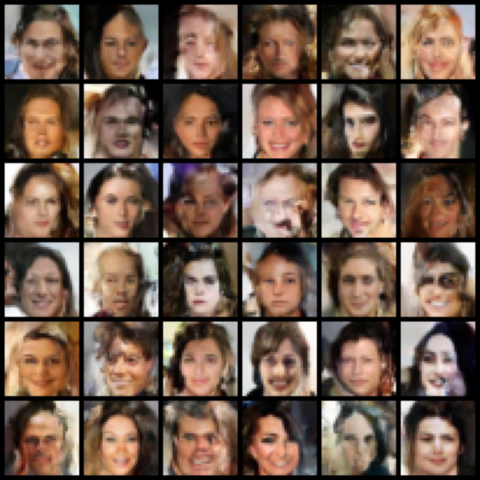
This is what the model generates after training for 50 epochs on the CelebA dataset.

For generating CIFAR10 images run:

model = torch.load("realnvp_CIFAR10.pt")
imgs = model.sample(n=36)  # img,shape = (36, 3, 32, 32)
grid = torchvision.utils.make_grid(imgs, nrow=6)
plt.imshow(grid.permute(1, 2, 0))

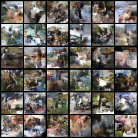
This is what the model generates after training for 350 epochs on the CIFAR10 dataset.

pi-tau / realnvp