Tools to enable flexible and efficient hierarchical nowcasting of right-truncated epidemiological time-series using a semi-mechanistic Bayesian model with support for a range of reporting and generative processes. Nowcasting, in this context, is gaining situational awareness using currently available observations and the reporting patterns of historical observations. This can be useful when tracking the spread of infectious disease in real-time: without nowcasting, changes in trends can be obfuscated by partial reporting or their detection may be delayed due to the use of simpler methods like truncation. While the package has been designed with epidemiological applications in mind, it could be applied to any set of right-truncated time-series count data.
Install the stable development version of the package with:
install.packages("epinowcast", repos = "https://epiforecasts.r-universe.dev")Alternatively, install the stable development from GitHub using the following,
remotes::install_github("epiforecasts/epinowcast", dependencies = TRUE)The unstable development version can also be installed from GitHub using the following,
remotes::install_github("epiforecasts/epinowcast@develop", dependencies = TRUE)If you don’t already have CmdStan installed then, in addition to
installing epinowcast, it is also necessary to install CmdStan using
CmdStanR’s install_cmdstan() function to enable model fitting in
epinowcast. A suitable C++ toolchain is also required. Instructions
are provided in the Getting started with
CmdStanR
vignette. See the CmdStanR
documentation for further details and
support.
cmdstanr::install_cmdstan()In this quick start we use COVID-19 hospitalisations by date of positive
test in Germany available up to the 1st of October 2021 to demonstrate
the specification and fitting of a simple nowcasting model using
epinowcast. Examples using more complex models are available in the
package vignettes and in the papers linked to in the literature
vignette.
As well as epinowcast this quick start makes use of data.table and
ggplot2 which are both installed when epinowcast is installed.
library(epinowcast)
library(data.table)
library(ggplot2)Nowcasting is effectively the estimation of reporting patterns for
recently reported data. This requires data on these patterns for
previous observations and typically this means the time series of data
as reported on multiple consecutive days (in theory non-consecutive days
could be used but this is not yet supported in epinowcast). For this
quick start these data are sourced from the Robert Koch Institute via
the Germany Nowcasting
hub
where they are deconvolved from weekly data and days with negative
reported hospitalisations are adjusted.
Below we first filter for a snapshot of retrospective data available 40 days before the 1st of October that contains 40 days of data and then produce the nowcast target based on the latest available hospitalisations by date of positive test.
nat_germany_hosp <-
  germany_covid19_hosp[location == "DE"][age_group %in% "00+"] |>
  enw_filter_report_dates(latest_date = "2021-10-01")

retro_nat_germany <- nat_germany_hosp |>
  enw_filter_report_dates(remove_days = 40) |>
  enw_filter_reference_dates(include_days = 40)
retro_nat_germany
#>      reference_date location age_group confirm report_date
#>   1:     2021-07-13       DE       00+      21  2021-07-13
#>   2:     2021-07-14       DE       00+      22  2021-07-14
#>   3:     2021-07-15       DE       00+      28  2021-07-15
#>   4:     2021-07-16       DE       00+      19  2021-07-16
#>   5:     2021-07-17       DE       00+      20  2021-07-17
#>  ---
#> 857:     2021-07-14       DE       00+      72  2021-08-21
#> 858:     2021-07-15       DE       00+      69  2021-08-22
#> 859:     2021-07-13       DE       00+      59  2021-08-21
#> 860:     2021-07-14       DE       00+      72  2021-08-22
#> 861:     2021-07-13       DE       00+      59  2021-08-22
latest_germany_hosp <- nat_germany_hosp |>
enw_latest_data() |>
enw_filter_reference_dates(remove_days = 40, include_days = 40)
head(latest_germany_hosp, n = 10)
#> reference_date location age_group confirm report_date
#> 1: 2021-07-13 DE 00+ 60 2021-10-01
#> 2: 2021-07-14 DE 00+ 74 2021-10-01
#> 3: 2021-07-15 DE 00+ 69 2021-10-01
#> 4: 2021-07-16 DE 00+ 49 2021-10-01
#> 5: 2021-07-17 DE 00+ 67 2021-10-01
#> 6: 2021-07-18 DE 00+ 51 2021-10-01
#> 7: 2021-07-19 DE 00+ 36 2021-10-01
#> 8: 2021-07-20 DE 00+ 96 2021-10-01
#> 9: 2021-07-21 DE 00+ 94 2021-10-01
#> 10: 2021-07-22 DE 00+ 99 2021-10-01Process reported data into format required for epinowcast and return
in a data.table. At this stage specify grouping (i.e age, location) if
any. It can be useful to check this output before beginning to model to
make sure everything is as expected.
pobs <- enw_preprocess_data(retro_nat_germany, max_delay = 40)
pobs
#>                    obs          new_confirm              latest
#> 1: <data.table[860x9]> <data.table[860x11]> <data.table[41x10]>
#>    missing_reference  reporting_triangle      metareference          metareport
#> 1: <data.table[0x6]> <data.table[41x42]> <data.table[41x9]> <data.table[80x12]>
#>             metadelay time snapshots by groups max_delay   max_date
#> 1: <data.table[40x4]>   41        41         1        40 2021-08-22
Construct a parametric lognormal intercept only model for the date of
reference using the metadata produced by enw_preprocess_data(). Note
that epinowcast uses a sparse design matrix for parametric delay
distributions to reduce runtimes so the design matrix shows only unique
rows with index containing the mapping to the full design matrix.
reference_module <- enw_reference(~1, distribution = "lognormal", data = pobs)Construct a model with a random effect for the day of report using the
metadata produced by enw_preprocess_data().
report_module <- enw_report(~ (1 | day_of_week), data = pobs)First compile the model. This step can be left to epinowcast but here
we want to use multiple cores per chain to speed up model fitting and so
need to compile the model with this feature turned on.
model <- enw_model(threads = TRUE)We now fit the model and produce a nowcast using this fit. Note that here we use two chains each using two threads as a demonstration but in general using 4 chains is recommended. Also note that warm-up and sampling iterations have been set below default values to reduce compute requirements but this may not be sufficient for many real world use cases. Finally, note that here we have silenced fitting progress and potential warning messages for the purposes of keeping this quick start short but in general this should not be done.
options(mc.cores = 2)
nowcast <- epinowcast(pobs,
  reference = reference_module,
  report = report_module,
  fit = enw_fit_opts(,
    save_warmup = FALSE, pp = TRUE,
    chains = 2, threads_per_chain = 2,
    iter_sampling = 500, iter_warmup = 500,
    show_messages = FALSE, refresh = 0
  ),
  model = model
)
#> Running MCMC with 2 parallel chains, with 2 thread(s) per chain...
#>
#> Chain 2 finished in 65.5 seconds.
#> Chain 1 finished in 77.3 seconds.
#>
#> Both chains finished successfully.
#> Mean chain execution time: 71.4 seconds.
#> Total execution time: 77.3 seconds.Print the output from epinowcast which includes diagnostic
information, the data used for fitting, and the cmdstanr object.
nowcast
#>                    obs          new_confirm              latest
#> 1: <data.table[860x9]> <data.table[860x11]> <data.table[41x10]>
#>    missing_reference  reporting_triangle      metareference          metareport
#> 1: <data.table[0x6]> <data.table[41x42]> <data.table[41x9]> <data.table[80x12]>
#>             metadelay time snapshots by groups max_delay   max_date
#> 1: <data.table[40x4]>   41        41         1        40 2021-08-22
#>                  fit       data  fit_args samples max_rhat
#> 1: <CmdStanMCMC[32]> <list[52]> <list[8]>    1000     1.02
#>    divergent_transitions per_divergent_transitions max_treedepth
#> 1:                     0                         0             8
#>    no_at_max_treedepth per_at_max_treedepth run_time
#> 1:                   5                0.005     77.3
Summarise the nowcast for the latest snapshot of data.
nowcast |>
  summary(probs = c(0.05, 0.95)) |>
  head(n = 10)
#>     reference_date report_date .group max_confirm location age_group confirm
#>  1:     2021-07-14  2021-08-22      1          72       DE       00+      72
#>  2:     2021-07-15  2021-08-22      1          69       DE       00+      69
#>  3:     2021-07-16  2021-08-22      1          47       DE       00+      47
#>  4:     2021-07-17  2021-08-22      1          65       DE       00+      65
#>  5:     2021-07-18  2021-08-22      1          50       DE       00+      50
#>  6:     2021-07-19  2021-08-22      1          36       DE       00+      36
#>  7:     2021-07-20  2021-08-22      1          94       DE       00+      94
#>  8:     2021-07-21  2021-08-22      1          91       DE       00+      91
#>  9:     2021-07-22  2021-08-22      1          99       DE       00+      99
#> 10:     2021-07-23  2021-08-22      1          86       DE       00+      86
#>     cum_prop_reported delay prop_reported    mean median        sd    mad q5
#>  1:                 1    39             0  72.000     72 0.0000000 0.0000 72
#>  2:                 1    38             0  69.032     69 0.1816838 0.0000 69
#>  3:                 1    37             0  47.083     47 0.2796233 0.0000 47
#>  4:                 1    36             0  65.218     65 0.4865313 0.0000 65
#>  5:                 1    35             0  50.264     50 0.5163047 0.0000 50
#>  6:                 1    34             0  36.246     36 0.4957113 0.0000 36
#>  7:                 1    33             0  94.462     94 0.6833908 0.0000 94
#>  8:                 1    32             0  91.706     91 0.8845034 0.0000 91
#>  9:                 1    31             0 100.074    100 1.1035134 1.4826 99
#> 10:                 1    30             0  87.203     87 1.1493964 1.4826 86
#>     q95      rhat  ess_bulk  ess_tail
#>  1:  72        NA        NA        NA
#>  2:  69 1.0036652 1002.1341 1000.1203
#>  3:  48 0.9982150  955.3026  949.0821
#>  4:  66 0.9984208  956.4874  936.4123
#>  5:  51 1.0012658  959.6633  845.4600
#>  6:  37 0.9990564  893.7362  875.3805
#>  7:  96 0.9993801  587.1606  617.8809
#>  8:  93 1.0017126 1049.6453 1010.8469
#>  9: 102 0.9991004 1013.5419  884.5519
#> 10:  89 0.9994546  849.4900  744.0604
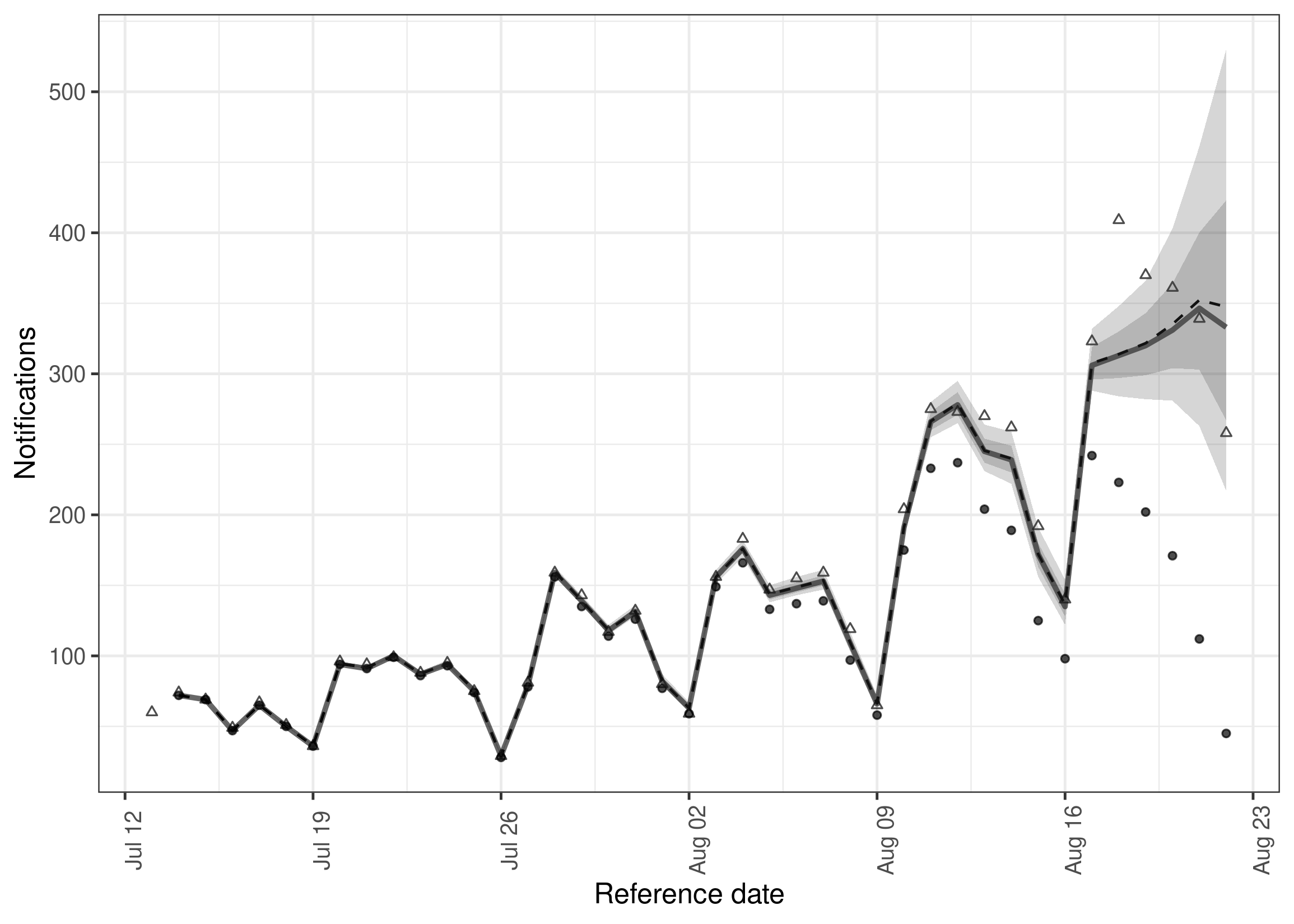
Plot the summarised nowcast against currently observed data (or optionally more recent data for comparison purposes).
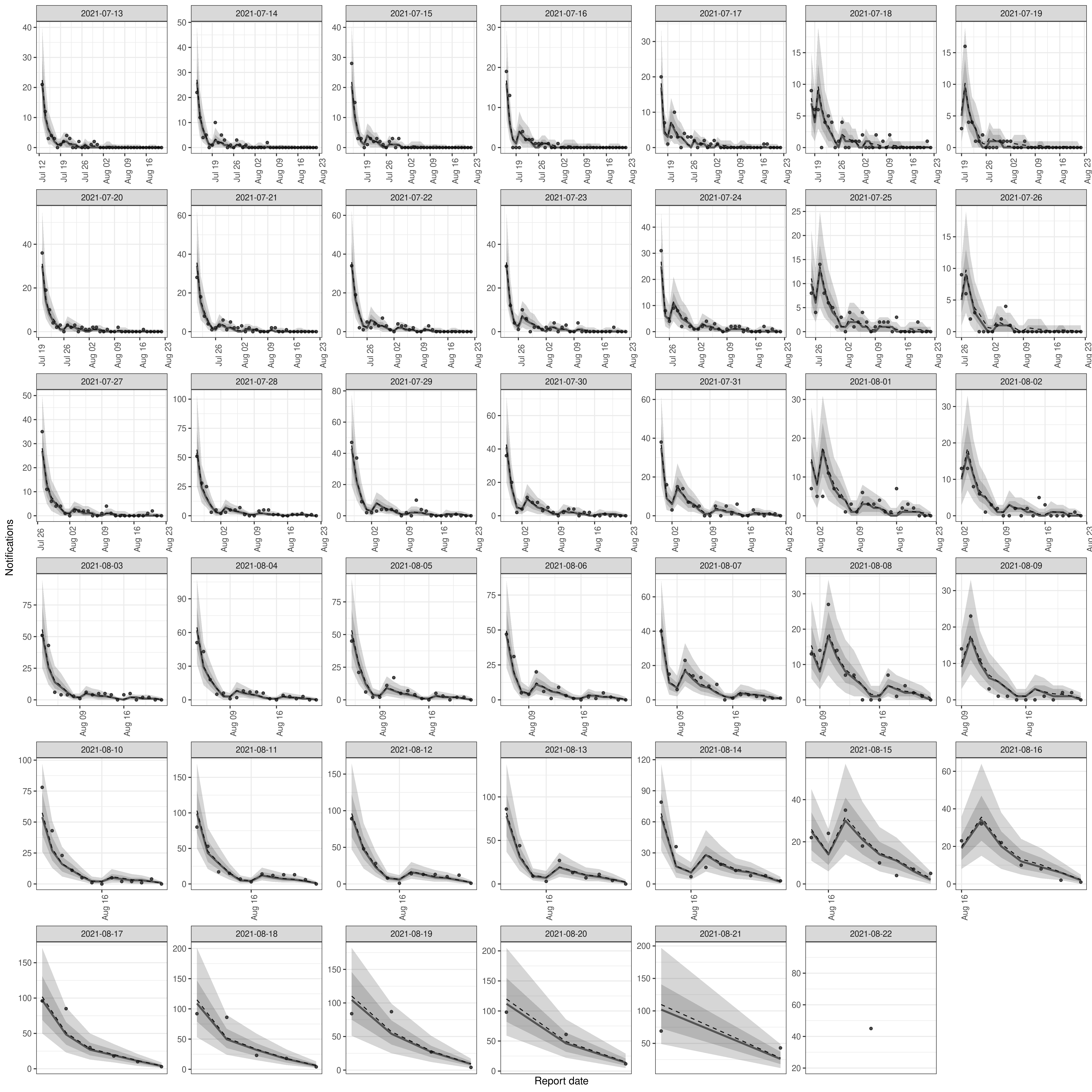
plot(nowcast, latest_obs = latest_germany_hosp)Plot posterior predictions for observed notifications by date of report as a check of how well the model reproduces the observed data.
plot(nowcast, type = "posterior") +
  facet_wrap(vars(reference_date), scale = "free")
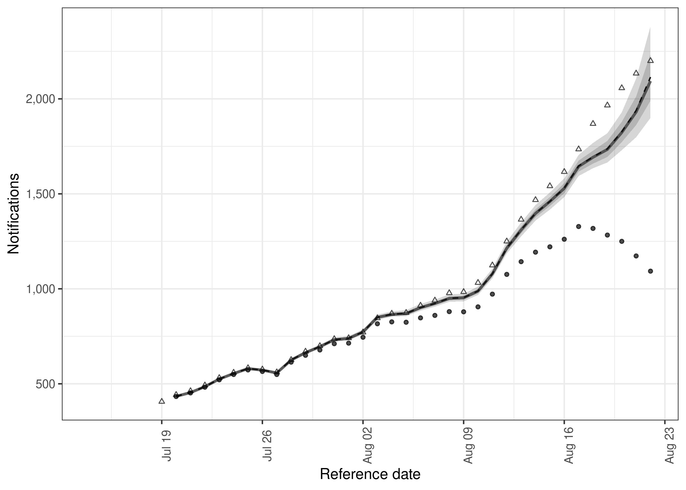
Rather than using the methods supplied for epinowcast directly,
package functions can also be used to extract nowcast posterior samples,
summarise them, and then plot them. This is demonstrated here by
plotting the 7 day incidence for hospitalisations.
# extract samples
samples <- summary(nowcast, type = "nowcast_samples")

# Take a 7 day rolling sum of both samples and observations
cols <- c("confirm", "sample")
samples[, (cols) := lapply(.SD, frollsum, n = 7),
  .SDcols = cols, by = ".draw"
][!is.na(sample)]
#>        reference_date report_date .group max_confirm location age_group confirm
#>     1:     2021-07-20  2021-08-22      1          94       DE       00+     433
#>     2:     2021-07-20  2021-08-22      1          94       DE       00+     433
#>     3:     2021-07-20  2021-08-22      1          94       DE       00+     433
#>     4:     2021-07-20  2021-08-22      1          94       DE       00+     433
#>     5:     2021-07-20  2021-08-22      1          94       DE       00+     433
#>    ---
#> 33996:     2021-08-22  2021-08-22      1          45       DE       00+    1093
#> 33997:     2021-08-22  2021-08-22      1          45       DE       00+    1093
#> 33998:     2021-08-22  2021-08-22      1          45       DE       00+    1093
#> 33999:     2021-08-22  2021-08-22      1          45       DE       00+    1093
#> 34000:     2021-08-22  2021-08-22      1          45       DE       00+    1093
#>        cum_prop_reported delay prop_reported .chain .iteration .draw sample
#>     1:                 1    33             0      1          1     1    435
#>     2:                 1    33             0      1          2     2    433
#>     3:                 1    33             0      1          3     3    436
#>     4:                 1    33             0      1          4     4    433
#>     5:                 1    33             0      1          5     5    433
#>    ---
#> 33996:                 1     0             1      2        496   996   1960
#> 33997:                 1     0             1      2        497   997   2253
#> 33998:                 1     0             1      2        498   998   1992
#> 33999:                 1     0             1      2        499   999   2014
#> 34000:                 1     0             1      2        500  1000   2069
latest_germany_hosp_7day <- copy(latest_germany_hosp)[
  ,
  confirm := frollsum(confirm, n = 7)
][!is.na(confirm)]

# Summarise samples
sum_across_last_7_days <- enw_summarise_samples(samples)

# Plot samples
enw_plot_nowcast_quantiles(sum_across_last_7_days, latest_germany_hosp_7day)The package has extensive documentation as well as vignettes describing the underlying methodology, and several case studies. Please see the package site for details. Note that the development version of the package also has supporting documentation which are available here.
If using epinowcast in your work please consider citing it using the
following,
#>
#> To cite epinowcast in publications use:
#>
#>   Sam Abbott, Adrian Lison, and Sebastian Funk (2021). epinowcast:
#>   Flexible hierarchical nowcasting, DOI: 10.5281/zenodo.5637165
#>
#> A BibTeX entry for LaTeX users is
#>
#>   @Article{,
#>     title = {epinowcast: Flexible hierarchical nowcasting},
#>     author = {Sam Abbott and Adrian Lison and Sebastian Funk},
#>     journal = {Zenodo},
#>     year = {2021},
#>     doi = {10.5281/zenodo.5637165},
#>   }
Please briefly describe your problem and what output you expect in an issue. If you have a question, please don’t open an issue. Instead, ask on our Q and A page. See our contributing guide for more information.
We welcome contributions and new contributors! We particularly appreciate help on priority problems in the issues. Please check and add to the issues, and/or add a pull request. See our contributing guide for more information.
If interested in expanding the functionality of the underlying model
note that epinowcast allows users to pass in their own models meaning
that alternative parameterisations, for example altering the forecast
model used for inferring expected observations, may be easily tested
within the package infrastructure. Once this testing has been done
alterations that increase the flexibility of the package model and
improves its defaults are very welcome via pull request or other
communication with the package authors. Even if not wanting to add your
updated model to the package please do reach out as we would love to
hear about your use case.
Please note that the epinowcast project is released with a
Contributor Code of
Conduct. By
contributing to this project, you agree to abide by its terms.


