CarND: Unscented Kalman Filter

The goal of this project is to develop a complete sensor fusion model, based on the Unscented Kalman Filter (UKF), in order to esimate the state of a moving vehicle combining measurments from two different types of sensors: lidar and radar.

UKF is an alternative technique to deal with non-linear process and measurement models. In many cases, the UKF approach approximates the non-linear transition better than linearization does. Furthermore, it does not require to compute Jacobian matrices.

The Motion Model

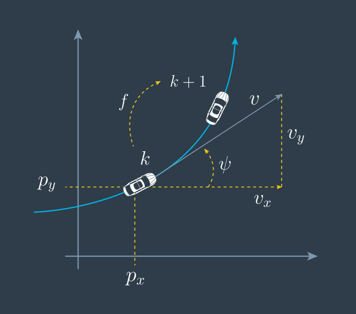
In this project, we will take advantage of the UKF by applying a more complex motion model than the Constant Velocity model used for the Extended Kalman Filter project: the Constant Turn Rate and Velocity Magnitude model (CTRV).

The State Vector

The state of the moving object is characterised by its 2D position x and y, the magnitude of the velocity v, the yaw angle psi that measures the orientation of the velocity vector, and the yaw rate psi_dot. Hence, the state vecor is [px, py, v, psi, psi_dot].

The State Transition

The integration of the differential motion model equations between two subsequent time steps yield a non-linear process function of the state vector.

Since the motion model assumes the velocity v and yaw rate psi_dot are constant between time intervals, accelerations are included in the model as random noise. Note that the bigger the time interval dt, the bigger the uncertainty introduced by the acceleration noise terms.

The Unscented Transformation

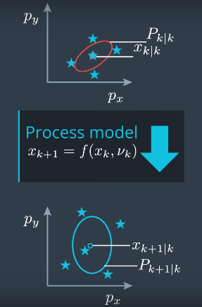
The objective is to transform a normal distribution, characterised by its mean vector and covariance matrix, via a non-linear function.

Rather than transforming the whole state distribution through the non-linear function, only a (small) set of special points are transformed: the sigma points. The sigma points are chosen around the mean state and in certain relation to the covariance of the distribution, serving as representatives of the whole distribution.

Each of one of the sigma points is transformed with the non-linear function, spanning on the predicted state space. Finally, the mean and covariance of the group of transformed sigma points can be calculated, yielding an approximation for the mean and covariance of the predicted distribution, treated as if it was normal (it is actually not because of the non-linearity).

Processing Flow Overview

The UKF algorithm iterates over a prediction-update loop as explained in the following sections.

0. Initialization

In the very first iteration of the algorithm, an initialization step replaces the prediction-update combo. The state of the vehicle is initialized with the help of the first set of incoming measurments. Laser measurements only provide information about px and py. Similarly, radar only determines completely the px and py positions, and only provides partial information about the initial velocity v through the radial projection rho_dot.

In the laser case, velocity was set horizontal, with no yaw acceleration: v = 5, yaw = 0, yaw_dot = 0, representing an initial moderate horizontal velocity. For initialization with radar measurements, v = rho_dot, yaw = 0, yaw_dot = 0; in absence of any information on the tangential velocity component, this is a reasonable option.

In any case, the state covariance matrix P was conveniently initialized to reflect the uncertainty of the initial estimates.

//laser
P_.fill(0.0);
P_(0,0) = std_laspx_*std_laspx_;
P_(1,1) = std_laspy_*std_laspy_;
P_(2,2) = 5*5;
P_(3,3) = M_PI*M_PI;
P_(4,4) = 0.1*0.1;
...
//radar 
P_.fill(0.0);
P_(0,0) = std_radr_*std_radr_;
P_(1,1) = std_radr_*std_radr_;
P_(2,2) = rho_dot*rho_dot;
P_(3,3) = M_PI*M_PI;
P_(4,4) = 0.1*0.1;

1. Prediction

The objective is to predict the mean and covariance for the next time step, state k+1|k (also known as the a priori estimation).

In order to evaluate the non-linear motion model, the unscented transformation is applied:

Generate sigma points for augmented state. Implemented in UKF::AugmentedSigmaPoints().
Apply the process function to the augmented sigma points. Implemented in UKF::SigmaPointPrediction().
Reconstruct the a priori state, x(k+1|k) and P(k+1|k), from the predicted sigma points. Implemented in UKF::PredictMeanAndCovariance().

2. Update

For both lidar and radar measurements, the update step consists of:

Apply the measurement model transformation to state k+1|k (given by the predicted sigma points from the previous step) to get the predicted measurements. Implemented in UKF::PredictLidarMeasurement() and UKF::PredictRadarMeasurement for laser and radar measurements respectively.
Calculate posterior state k+1|k+1. Implemented in UKF::UpdateState().

Finally, for the eventual consistency check, the Normalized Innovation Squared (NIS) is calculated, using UKF::CalculateNIS().

Consistency

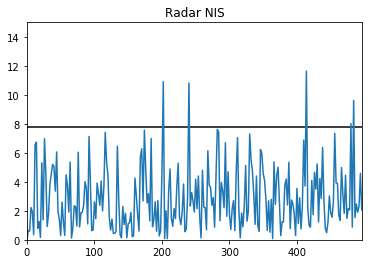
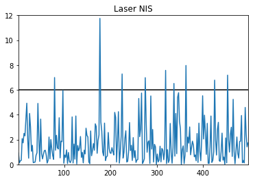
The noise parameters and initialization process were tweaked in order to make the system consistent. This was checked by means of a NIS test for radar and laser measurents:

Performance Evaluation

The ground truth positions for each instant are available. Thus, the performance of the tracking algorithm is evaluated with the Root Mean Squared Error (RMSE), an accuracy metric that measures the deviation of the estimated state from the true state.

The initialization of the state vector and covariance matrix was tweaked to yield [px, py, vx, vy] RMSEs bellow [.09, .10, .40, .30] throughout most of the simulation.

Note that [px, py, vx, vy] is not the state vector used for this project. Nevertheless, this state vector can be easily inferred, as done in main.cpp:

double px = ukf.x_(0);
double py = ukf.x_(1);
double v  = ukf.x_(2);
double yaw = ukf.x_(3);
double yaw_dot = ukf.x_(4);

double vx = cos(yaw)*v;
double vy = sin(yaw)*v;

Conclusion

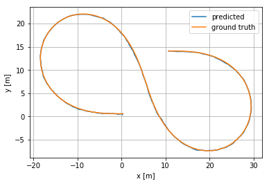
The Unscented Kalman Filter was tuned aiming for consistency, and succesfully managed to locate a moving vehicle:

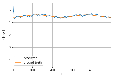
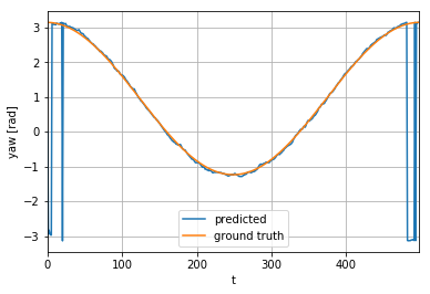
One of the most fascinating capabilities of the UKF, is that it is able to predict accurately underlying state variables that are not even provided by sensors, such as velocity and yaw:

partmor / SDC-Unscented-Kalman-Filter