CarND: Behavioral Cloning

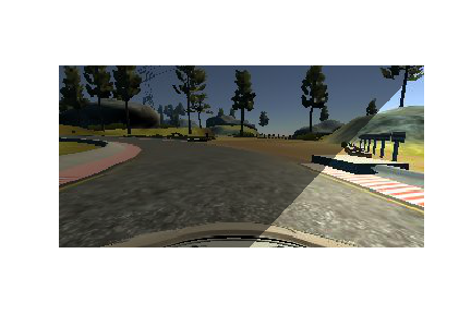
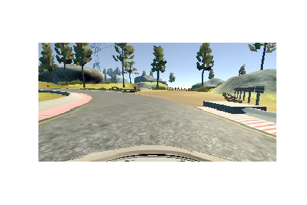
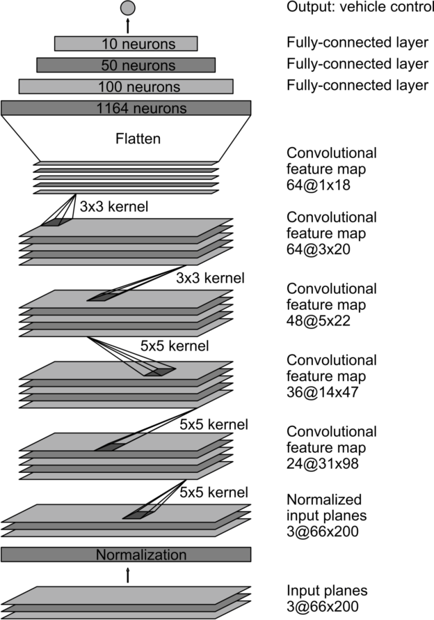
The goal of this project is to train a convolutional neural network (CNN) based model, using an end-to-end approach: raw pixels from a front-facing camera are mapped to the steering commands for a self-driving car.

The data of good driving behaviour is collected driving a car around a track in a simulator. A CNN built with Keras is trained with the latter data to predict steering angles from images. Eventually this model is assessed by testing it successfully drives around the track without leaving the road.

Project structure

The project includes the following files:

File	Description
`data_manipulation.py`	Contains methods for data loading, balancing, and augmentation.
`model.py`	Definition of the model architecture and training process.
`model.h5`	Contains the trained model outputed in `model.py`
`drive.py`	In autonomous mode, it communicates with the driving simulator guiding the car based on real time predictions provided by `model.h5`.

Details about the files

The model is built, trained and saved with the following command:

python model.py

and once the simulator app is set to Autonomous Mode, the prediction stream is established executing:

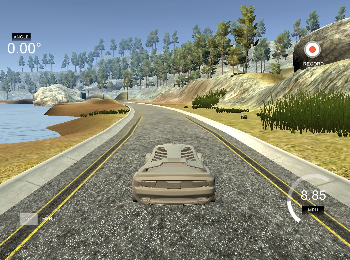
python drive.py model.h5

Data collection

The driving simulator saves frames from the car's point of view corresponding to three front-facing cameras, together with the state of the vehicle: throttle, speed and steering angle.

The training data for the CNN is collected from track 1. The car is driven safelly around the track, always focusing on keeping the car in the center of the lane.

To help the model generalize better, the following actions are performed during data collection:

Completing laps in both clockwise and counter-clockwise directions, accomplishing a higher balance of left/right curves.
Record forced recovery scenarios: taking the car intentionally out of the path and recording just the recovery maneuver. This will increase the model's robustness against perturbations and help the model learn to take U-turns, despite there are none in this circuit.

Drive extra laps just recording through curves.

Data balancing

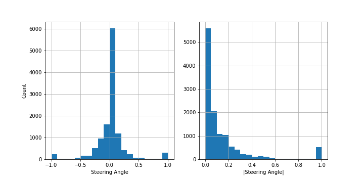
In spite of following the described methodology for data collection, the dataset is still unbalanced:

According to the figure above, if trained with the dataset as is, the model will be biased to driving in a straight line, something we want to avoid.

Balancing is performed by sublampling the dataset; the samples are binned based on the absolute value of the steering angle, and bin size is restricted to be lower than an given amount thresh:

def get_balanced_dataset_indices(dataset, num_bins, thresh='mean'):
    selection_list = list()

    # the data is balanced based on the absolute value steering angle
    y = dataset['steering']
    y_abs = np.abs(y)

    # binning of the measurements
    hist, bins = np.histogram(y_abs, bins=num_bins)
    bin_idx = np.digitize(np.abs(y), bins=bins)
    if thresh=='mean':
        thresh = hist.mean()
    
    # for each bin pick a random subsample of a maximum size given by `thresh`
    for a, b in zip(np.roll(bins, shift=1)[1:], bins[1:]):
        idx_in_bin = y[(y_abs > a) & (y_abs <= b)].index
        if len(idx_in_bin) > 0:
            subset = np.random.choice(idx_in_bin, size=min(int(thresh), len(idx_in_bin)), replace=False)
            selection_list.append(subset)
    
    # return the indices of the balanced data
    selected_idx = np.concatenate(selection_list)
    return selected_idx

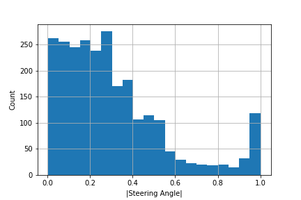
Using this method, the original unbalanced dataset with 12146 samples is downsampled to 2537 using num_bins=50 and thresh=100, now with the following distribution:

Bear in mind that balancing is performed across absolute values, since applying horizontal flip during augmentation will mitigate potential small unbalances between left/right turns.

Data augmentation

Tha data balancing from the latter step yielded a 2.5k sample dataset that is clearly insufficient to train a model that could generalize well. However, the following augmentation techniques altogether enable the extension of the dataset by an order of magnitude:

Left and right cameras: each collected sample includes images taken from 3 camera positions: left, center and right. During the autonomous driving stage (test) the only input will be the center camera frame. However, the lateral cameras can still be used for training (selecting position randomly) by applying a correction corr_angle to the associated steering angle. This increases samples by a factor of 3.

cameras = {
    0: 'left_img',
    1: 'center_img',
    2: 'right_img'
}

angle_correction = {
    0: corr_angle,
    1: 0.0,
    2: - corr_angle
}
...
...
# randomly select between left/center/right cameras and apply corresponding correction
cam = np.random.randint(3) if use_lat else 1
# use regex to be able to read paths with normal slash and backslash
img_fname = '%sIMG/%s' % (samples_folder,  re.compile(r'/|\\').split(batch_sample[cameras[cam]])[-1])
image = imread(img_fname)
angle = batch_sample['steering'] + angle_correction[cam]

Horizontal flip: frames are horizontally flipped at random, together with a change in the sign of the steering angle. This increases samples by a factor of 2.

# randomly decide whether to flip or not the image
if np.random.choice([True, False]):
    image = np.fliplr(image)
    angle = - angle

Random shadow: a random slice shadowing of the image is performed, by decreasing brightness of a random frame slice, hoping to make the model robust against shadows, marks, and texture variation on the road.

def apply_random_section_shading(img):
    h, w = img.shape[0], img.shape[1]
    [x1, x2] = np.random.choice(w, 2, replace=False)
    k = h / (x2 - x1)
    b = - k * x1
    for i in range(h):
        c = int((i - b) / k)
        img[i, :c, :] = (img[i, :c, :] * .5).astype(np.uint8)
    return img

Random brightness: the brightness of the image is altered using a range of random values for gamma adjustment. The objective is to also increase robustness against lighting conditions and tarmac tonalities.

def apply_random_gamma_adjust(img, low, high):
    gamma = np.random.random_sample() * (high - low) + low
    return adjust_gamma(img, gamma=gamma)

These augmentation techniques are encapsulated in a pipeline to work as a generator (batch_generator method in data_manipulation.py), allowing to augment the data real-time, without having to worry about running out of memory for instance.

Following this pipeline, the original dataset can be effectively augmented at least by a factor of 6, while also enhancing the robustness of the model by pertubing the images.

All the augmentation steps except horizontal flip are disabled to generate the validation set.

Preprocessing

Training, validation, and eventually test data, run through a common pipeline that comprises:

YUV colorspace transformation: the images are converted from RGB to YUV colorspace, after the augmentation pipeline in the training phase, and during collection (within drive.py) in the testing phase. This is accomplished with the helper method out_of_pipeline_preprocessing in data_manipulation.py. The YUV colorspace was used in NVIDIA's end-to-end deep learning for self-driving cars project. This election is supported by the added robustness that this colorspace provides for detecting features in images for automotive applications, since varying lighting conditions are isolated effectively by the luma Y channel, from the color information enclosed in the U and V channels. The usage of this colorspace could somehow reduce the effectiveness of the brightness transformation augmentation-step.
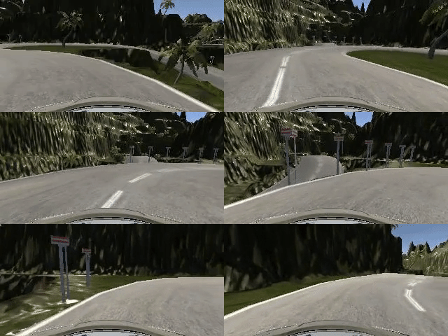
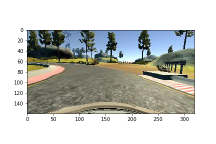
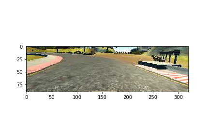
Image cropping: as seen in the image bellow, the raw frames collected by the camera have regions that provide little information and potentially just add noise; that is the landscape above the horizon of the lane, and the bonnet of the car. Cropping the top 60 rows and bottom 25 rows of pixels of the original image (160 x 320) can help the model focus on extracting the important lane features. This step is performed within the model with a Keras Cropping2D layer:

model.add(Cropping2D(cropping=((60,25), (0,0)), input_shape=(160,320,3)))

Scaling: scaling the input helps the convergence of the optimization algorithm during the training phase. A simple [0,1] scaling of the input pixels followed by a mean substraction is performed with a Keras Lambda layer:

model.add(Lambda(lambda x: (x / 255.0) - 0.5))

Model architecture

NVIDIA's CNN architecture was taken as a baseline in this project.

This architecture could be fairly over-dimensioned for the scope of this project: the data is collected from a circuit which is flat, does not have U-turns, tarmac texture is relatively constant, and most importantly, there are not any obstacles whatsoever in the path, e.g., other cars circulating.

Auto-driving on track 1 is relatively easy. First of all because the morphology and casuistry from this track is not very complex. Secondly, because the model has been trained on the same circuit, so it is basically a case of in-sample testing, which is not the most rigorous way to assess the performance of a model.

The first dense layer of 1164 neurons was removed. Testing on track 1 architectures with less convolution layers and added max pooling layers yielded very satisfactory results on this track, but were not flexible enough to generalize the hard recovery situations from track 1 to get over the U-turns in track 2.

Taking this into account, the architecture that best performed on both tracks is:

def build_Nvidia_Modified(model):
    model.add(Conv2D(24, kernel_size=(5, 5), strides=(2, 2), activation="relu"))
    model.add(Conv2D(36, kernel_size=(5, 5), strides=(2, 2), activation="relu"))
    model.add(Conv2D(48, kernel_size=(5, 5), strides=(2, 2), activation="relu"))
    model.add(Conv2D(64, kernel_size=(3, 3), activation="relu"))
    model.add(Conv2D(64, kernel_size=(3, 3), activation="relu"))
    model.add(Flatten())
    model.add(Dense(100, activation='relu'))
    model.add(Dense(50, activation='relu'))
    model.add(Dense(10, activation='relu'))
    model.add(Dense(1))

As said, it imitates NVIDIA's original architecture, but without the first 1164-neuron dense layer. Non-linearities are introduced using ReLU activations.

NOTE: A smaller regularized model is included in model.py, instantiated with the method build_Smaller(). This model can auto-drive perfectly around track 1, but not on track 2.

Model training

The balanced data set is split into a training and a validation set, following a 80-20 proportion.

As described, during the training phase, the training data is augmented real-time with the batch_generator defined in data_manipulation.py. Validation data is also fed into the training algorithm via batch_generator, but in this case only image flipping is enabled.

The objective loss function to minimize is the mean squared error over the training set. This function is optimized using Adam, a method that computes adaptive learning rates for each parameter.

IMPORTANT NOTE: Many combinations of dropout (0.5 - 1) on dense layers, and L2 penalty (several logarithmic scales: -1 to -4) on the dense layers and convolution kernels were tested. However, they ended up rigidizing the model in a way it could not drive through track 2 entirely without failing in the U-turns and/or the S-shaped slopes. Hence, the final model was finally trained without regularization.

The model successfully drove around tracks 1 and 2 after training for 5 epochs:

model.compile(loss='mse', optimizer='adam')
model.fit_generator(
    train_generator,
    steps_per_epoch=6*train_df.shape[0]/BATCH_SIZE,
    validation_data=valid_generator,
    validation_steps=2*valid_df.shape[0]/BATCH_SIZE,
    epochs=5
)

In order to extract the maximum benefit of data augmentation, in each epoch the training data is stepped through 6 times (recall the 2x and 3x augmentations provided by flipping and camera selection respectively) while the validation data is stepped through 2 times (2x flipping augmentation).

Results

The trained model managed to drive successfully around both tracks. The solution video files of the car driving a whole lap in autonomous mode for track 1 and 2 are included in this repo: video_track1_autodrive.mp4 and video_track2_autodrive.mp4 respectively.

The gif above shows one of the critical sections of track 2 (corresponding to minute 4:37 of video 2): a U-curve where another stretch of road can be seen in the horizon due to difference of level. The car could easilly think it should keep driving towards the road in the horizon, but does not, as intended.

Also, here are the YouTube links for video 1 and video 2.

partmor / SDC-Behavioral-Cloning