Classify hand-written digits from MNIST dataset using Tensorflow
import tensorflow as tf
import math
import numpy as np
import h5py
import matplotlib.pyplot as plt
import tensorflow as tf
from tensorflow.python.framework import ops

mnist = tf.keras.datasets.mnist

(x_train, y_train), (x_test, y_test) = mnist.load_data()
x_train, x_test = x_train / 255.0, x_test / 255.0
m = x_train.shape[0] # m is the total number of samples

print("m = " + str(m))

print("Shape of training data x_train: " + str(x_train.shape) + " y_train : " + str(y_train.shape))
print("Shape of test data : " + str(x_test.shape))
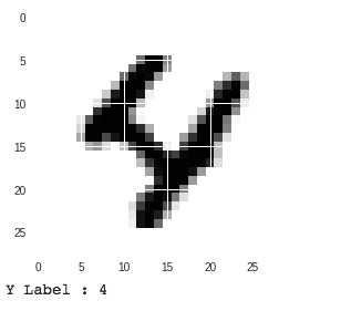
Print some random digits
%matplotlib inline
import matplotlib
import matplotlib.pyplot as plt

digit_index = 729
some_digit = x_train[digit_index]

plt.imshow(some_digit, cmap = matplotlib.cm.binary, interpolation="nearest")
#plt.axis("off")
plt.show()

print("Y Label : " + str(y_train[digit_index]))
Flatten the 2D images to 1D array
# Flatten the images from 2D to 1D
X_train_flatten = x_train.reshape(x_train.shape[0], -1).T
X_test_flatten = x_test.reshape(x_test.shape[0], -1).T
print("X_train_flatten shape = " + str(X_train_flatten.shape))
print("X_test_flatten shape = " + str(X_test_flatten.shape))
X_train_flatten shape = (784, 60000) X_test_flatten shape = (784, 10000)
Convert class label y to one hot vectors
# Convert each label to a vector of total_classes where only one index that corresponds to the label is one.
# Each label vector is a column vector
def one_hot_matrix(labels):

    # There are total 10 digits, thus, C that corresponds to total number of classes is 10
    C = tf.constant(10, name="C")
    one_hot_matrix = tf.one_hot(indices=labels, depth=C, axis=0)

    sess = tf.Session()
    one_hot = sess.run(one_hot_matrix)
    sess.close()

    return one_hot
# Convert y-labels to 1 hot representation
y_train_onehot = one_hot_matrix(y_train)
y_test_onehot = one_hot_matrix(y_test)
print("Shape of y_train_onehot : " + str(y_train_onehot.shape))
print("Shape of y_test_onehot : " + str(y_test_onehot.shape))Shape of y_train_onehot : (10, 60000) Shape of y_test_onehot : (10, 10000)
Create Tensorflow placeholders
def create_placeholders(n_x, n_y):
    """
    Creates the placeholders for the tensorflow session.

    Arguments:
    n_x -- scalar, size of an image vector (num_px * num_px = 64 * 64 = 784)
    n_y -- scalar, number of classes (from 0 to 9, so -> 10)

    Returns:
    X -- placeholder for the data input, of shape [n_x, None] and dtype "float"
    Y -- placeholder for the input labels, of shape [n_y, None] and dtype "float"

    Tips:
    - You will use None because it let's us be flexible on the number of examples you will for the placeholders.
      In fact, the number of examples during test/train is different.
    """

    ### START CODE HERE ### (approx. 2 lines)
    X = tf.placeholder(tf.float32, shape = (n_x, None))
    Y = tf.placeholder(tf.float32, shape = (n_y, None))
    ### END CODE HERE ###

    return X, Y
Define a Neural network with 2 hidden layers. First hidden layer has 25 nodes, second has 12. ReLU is used as activation function for the hidden layers and softmax for the output layer.
# Initializes the parameters for the Neural network
# The neural network has 2 hidden layers with 25 nodes in the first layer and 12 nodes in the second layer
# The output layer has 10 nodes corresponding to the 10 output classes
def initialize_parameters():

    tf.set_random_seed(7)

    W1 = tf.get_variable("W1", shape=[25, 784], initializer = tf.contrib.layers.xavier_initializer())
    b1 = tf.get_variable("b1", [25, 1], initializer=tf.zeros_initializer())
    W2 = tf.get_variable("W2", [12, 25], initializer=tf.contrib.layers.xavier_initializer(seed = 1))
    b2 = tf.get_variable("b2", [12, 1], initializer=tf.zeros_initializer())
    W3 = tf.get_variable("W3", [10, 12], initializer = tf.contrib.layers.xavier_initializer(seed = 1))
    b3 = tf.get_variable("b3", [10,1], initializer = tf.zeros_initializer())

    parameters = {
        "W1": W1,
        "b1": b1,
        "W2": W2,
        "b2": b2,
        "W3": W3,
        "b3": b3
    }

    return parameters
# Implements the forward propagation in the neural network.
# For the 2 hidden layers, RELU is the activation function.
# For the output layer, there's no activation function.
# Actually, there's sigmoid function, but taken care of in the cost calculation
def forward_propagation(X, parameters):
W1 = parameters['W1']
b1 = parameters['b1']
W2 = parameters['W2']
b2 = parameters['b2']
W3 = parameters['W3']
b3 = parameters['b3']
Z1 = tf.add(tf.matmul(W1, X), b1)
A1 = tf.nn.relu(Z1)
Z2 = tf.add(tf.matmul(W2, Z1), b2)
A2 = tf.nn.relu(Z2)
Z3 = tf.add(tf.matmul(W3, Z2), b3)
return Z3Define the cost of the Neural network
# For the output layer, we use softmax activation function and calculate the overall cost.
# Z3 is the output from the last hidden layer
# Y is the "true" labels vector placeholder
def calculate_cost(Z3, Y):

    # Tensorflow expects the shape to be (num_examples, num_classes)
    # Hence, we need to transpose these two
    labels = tf.transpose(Y) # These correspond to y
    logits = tf.transpose(Z3) # These correspond to Z

    cost = tf.reduce_mean(tf.nn.softmax_cross_entropy_with_logits(logits = logits, labels = labels))

    return cost
Create a Tensorflow session
tf.reset_default_graph()

with tf.Session() as sess:
    X, Y = create_placeholders(784, 10)
    parameters = initialize_parameters()
    Z3 = forward_propagation(X, parameters)
    cost = calculate_cost(Z3, Y)
    print("cost = " + str(cost))
cost = Tensor("Mean:0", shape=(), dtype=float32)
Helper method to create random mini batches
def random_mini_batches(X, Y, mini_batch_size = 64, seed = 0):
    """
    Creates a list of random minibatches from (X, Y)

    Arguments:
    X -- input data, of shape (input size, number of examples)
    Y -- true "label" vector (containing 0 if cat, 1 if non-cat), of shape (1, number of examples)
    mini_batch_size - size of the mini-batches, integer
    seed -- this is only for the purpose of grading, so that you're "random minibatches are the same as ours.

    Returns:
    mini_batches -- list of synchronous (mini_batch_X, mini_batch_Y)
    """

    m = X.shape[1]                  # number of training examples
    mini_batches = []
    np.random.seed(seed)

    # Step 1: Shuffle (X, Y)
    permutation = list(np.random.permutation(m))
    shuffled_X = X[:, permutation]
    shuffled_Y = Y[:, permutation].reshape((Y.shape[0],m))

    # Step 2: Partition (shuffled_X, shuffled_Y). Minus the end case.
    num_complete_minibatches = math.floor(m/mini_batch_size) # number of mini batches of size mini_batch_size in your partitionning
    for k in range(0, num_complete_minibatches):
        mini_batch_X = shuffled_X[:, k * mini_batch_size : k * mini_batch_size + mini_batch_size]
        mini_batch_Y = shuffled_Y[:, k * mini_batch_size : k * mini_batch_size + mini_batch_size]
        mini_batch = (mini_batch_X, mini_batch_Y)
        mini_batches.append(mini_batch)

    # Handling the end case (last mini-batch < mini_batch_size)
    if m % mini_batch_size != 0:
        mini_batch_X = shuffled_X[:, num_complete_minibatches * mini_batch_size : m]
        mini_batch_Y = shuffled_Y[:, num_complete_minibatches * mini_batch_size : m]
        mini_batch = (mini_batch_X, mini_batch_Y)
        mini_batches.append(mini_batch)

    return mini_batches
Create the model using the previously defined functions
# Now we build the main neural network using the previously built functions

def model(X_train, Y_train, X_test, Y_test, learning_rate=0.0001,
         num_epochs = 200, minibatch_size=32, print_cost=True):

    ops.reset_default_graph()

    tf.set_random_seed(7)
    seed = 3
    (n_x, m) = X_train.shape # Get the number of features and training samples
    n_y = Y_train.shape[0]

    costs = [] # To keep track of the costs

    # Create placeholders for X and Y
    X, Y = create_placeholders(n_x, n_y)

    # Initialize the W and b parameters for all the layers
    parameters = initialize_parameters()

    # Forward propagation
    Z3 = forward_propagation(X, parameters)

    # Calcualte the cost in forward propagation
    cost = calculate_cost(Z3, Y)

    # Backpropagation: Define the tensorflow optimizer. Use an AdamOptimizer.
    optimizer = tf.train.AdamOptimizer(learning_rate = learning_rate).minimize(cost)

    # Initialize all the variables
    init = tf.global_variables_initializer()

    # Start the tensorflow session
    with tf.Session() as sess:

        # Run the initialization
        sess.run(init)

        for epoch in range(num_epochs):

            epoch_cost = 0
            num_minibatches = int(m / minibatch_size) # number of minibatches of size minibatch_size in the train set
            seed = seed + 1
            minibatches = random_mini_batches(X_train, Y_train, minibatch_size, seed)

            for minibatch in minibatches:

                # Select a minibatch
                (minibatch_X, minibatch_Y) = minibatch

                # IMPORTANT: The line that runs the graph on a minibatch.
                # Run the session to execute the "optimizer" and the "cost", the feedict should contain a minibatch for (X,Y).
                ### START CODE HERE ### (1 line)
                _ , minibatch_cost = sess.run([optimizer, cost], feed_dict={X: minibatch_X, Y: minibatch_Y})
                ### END CODE HERE ###

                epoch_cost += minibatch_cost / num_minibatches

            # Print the cost every epoch
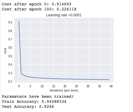
            if print_cost == True and epoch % 100 == 0:
                print ("Cost after epoch %i: %f" % (epoch, epoch_cost))
            if print_cost == True and epoch % 5 == 0:
                costs.append(epoch_cost)

        # plot the cost
        plt.plot(np.squeeze(costs))
        plt.ylabel('cost')
        plt.xlabel('iterations (per tens)')
        plt.title("Learning rate =" + str(learning_rate))
        plt.show()

        # lets save the parameters in a variable
        parameters = sess.run(parameters)
        print ("Parameters have been trained!")

        # Calculate the correct predictions
        correct_prediction = tf.equal(tf.argmax(Z3), tf.argmax(Y))

        # Calculate accuracy on the test set
        accuracy = tf.reduce_mean(tf.cast(correct_prediction, "float"))

        print ("Train Accuracy:", accuracy.eval({X: X_train, Y: Y_train}))
        print ("Test Accuracy:", accuracy.eval({X: X_test, Y: Y_test}))

        return parameters
parameters = model(X_train_flatten, y_train_onehot, X_test_flatten, y_test_onehot)
