This is a module to convert between one dimensional distance along a
Hilbert curve, h, and N-dimensional coordinates,
(x_0, x_1, ... x_N-1). The two important parameters are N
(the number of dimensions, must be > 0) and p (the number of
iterations used in constructing the Hilbert curve, must be > 0).
We consider an N-dimensional hypercube of side length 2^p.
This hypercube contains 2^{N p} unit hypercubes (2^p along
each dimension). The number of unit hypercubes determine the possible
discrete distances along the Hilbert curve (indexed from 0 to
2^{N p} - 1).
You can calculate coordinates given distances along a hilbert curve,
from hilbert import HilbertCurve
p=1; N=2
hilbert_curve = HilbertCurve(p, N)
for ii in range(4):
    coords = hilbert_curve.coordinates_from_distance(ii)
    print(f'coords(h={ii}) = {coords}')
coords(h=0) = [0, 0]
coords(h=1) = [0, 1]
coords(h=2) = [1, 1]
coords(h=3) = [1, 0]
You can also calculate distances along a hilbert curve given coordinates,
for coords in [[0,0], [0,1], [1,1], [1,0]]:
    dist = hilbert_curve.distance_from_coordinates(coords)
    print(f'distance(x={coords}) = {dist}')
distance(x=[0, 0]) = 0
distance(x=[0, 1]) = 1
distance(x=[1, 1]) = 2
distance(x=[1, 0]) = 3
Due to the magic of arbitrarily large integers in Python, these calculations can be done with ... well ... arbitrarily large integers!
p = 512; N = 10
hilbert_curve = HilbertCurve(p, N)
ii = 123456789101112131415161718192021222324252627282930
coords = hilbert_curve.coordinates_from_distance(ii)
print(f'coords = {coords}')
coords = [121075, 67332, 67326, 108879, 26637, 43346, 23848, 1551, 68130, 84004]
The calculations above represent the 512th iteration of the Hilbert curve in 10 dimensions. The maximum value along any coordinate axis is an integer with 155 digits and the maximum distance along the curve is an integer with 1542 digits. For comparison, an estimate of the number of atoms in the observable universe is 10**82 (i.e. an integer with 83 digits).

The figure above shows the first three iterations of the Hilbert
curve in two (N=2) dimensions. The p=1 iteration is shown
in red, p=2 in blue, and p=3 in black.
For the p=3 iteration, distances, h, along the curve are
labeled from 0 to 63 (i.e. from 0 to 2^{N p}-1). The hilbert module
provides methods to translate between N-dimensional coordinates and one
dimensional distance. For example, between (x_0=4, x_1=6) and
h=36.
Note that the p=1 and p=2 iterations have been scaled and translated
to the coordinate system of the p=3 iteration.
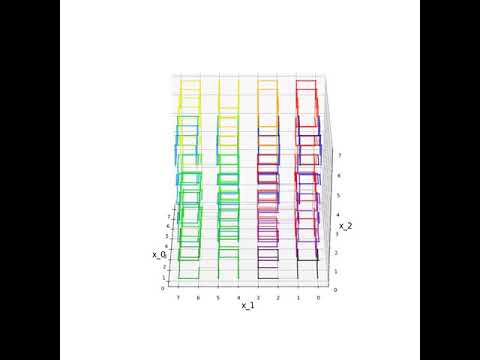
An animation of the same case in 3-D is available on YouTube. To watch the video, click the link below. Once the YouTube video loads, you can right click on it and turn "Loop" on to watch the curve rotate continuously.
This module is based on the C code provided in the 2004 article "Programming the Hilbert Curve" by John Skilling,
I was also helped by the discussion in the following stackoverflow post,
which points out a typo in the source code of the paper. The Skilling code
provides two functions TransposetoAxes and AxestoTranspose. In this
case, Transpose refers to a specific packing of the integer that represents
distance along the Hilbert curve (see below for details) and
Axes refer to the N-dimensional coordinates. Below is an excerpt from the
documentation of Skilling's code,
//+++++++++++++++++++++++++++ PUBLIC-DOMAIN SOFTWARE ++++++++++++++++++++++++++
// Functions: TransposetoAxes  AxestoTranspose
// Purpose:   Transform in-place between Hilbert transpose and geometrical axes
// Example:   b=5 bits for each of n=3 coordinates.
//            15-bit Hilbert integer = A B C D E F G H I J K L M N O is stored
//            as its Transpose
//                   X[0] = A D G J M                X[2]|
//                   X[1] = B E H K N    <------->       | /X[1]
//                   X[2] = C F I L O               axes |/
//                          high  low                    0------ X[0]
//            Axes are stored conveniently as b-bit integers.
// Author:    John Skilling  20 Apr 2001 to 11 Oct 2003