Implementation of 'An Image is Worth 16x16 Words: Transformers for Image Recognition at Scale' ICLR 2020 (arXiv, PDF)
and a documentation about its historical and technical background.
Some figures and equations are from their original paper.

- Preceding Works
- Attention Mechanism
- Transformers
- Vision Transformers
- Overall Structure
- Patching
- Positional Embedding
- Layer Normalization
- GELU Activation
- Experiments
- Environments
- Result
In the field of NLP, they pushed the limitations of RNNs by developing attention mechanism. Attention mechanism is a method to literally pay attention to the important features. In NLP, for example, with the sentence "I love NLP because it is fascinating.", the word 'it' referes to 'NLP'. Thus, when you process 'it', you have to treat it as 'NLP'.
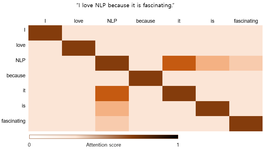
Figure1. An example of attention score between words in a sentence. You can see 'it' and 'NLP' has high attention score. This examples represents one of attention mechanisms called self-attention.

Attention is basically inner product operation as similarity measurement. You have three following informations:
| Acronym | Name | Description | En2Ko example |
|---|---|---|---|
| Q | Query | An information to compare this with all keys to find the best-matching key. | because |
| K | Key | A set of key that leads to appropriate values. | I, love, NLP, because, it, is, fascinating |
| V | Value | The result of attention. | 나, 자연어처리, 좋, 왜냐하면, 이것, 은, 흥미롭다 |
When you translate "because" in "I love NLP because it is fascinating.", first you calculate the similarity between "because" and other words. Then, weight-sum the korean words with the similarity, you get an appropriate word vector.
To take attention mechanism further, Ashish Vaswani et al. introduced a framework named called "Transformer". Transformer takes a sequential sentence as a pile of words and extracts features through attention encoder and decoders with several types of attention. More details of transformer structure is explained on the "Transformer" section. While attention mechanism sounds quite reasonable with NLP examples, it's not trivial that it works in computer vision as well. Alexey Dosovitskiy from Google Research introduced transformer for computer vision and explained how it works.
By attention mechanism, in NLP, the model calculates where to concentrate. On the other hand, in computer vision, Jie Hu et al. proposed a new attention structure for computer vision (Squeeze-and Excitation Networks, CVPR 2018, arXiv, PDF). The proposed architecture contains a sub-network that learns channel-wize attention score.
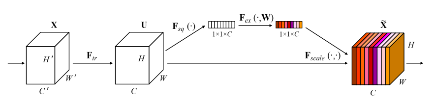
Figure2. This diagram shows the structure of squeeze-and-excitation module. A sub-network branch makes 1x1xC dimensional tensor of attention scores for the input of the module.

Convolutional neural networks, is in a way, a channel-level ensemble. Each kernels extracts different features from an image for another features. But these features from different kernels are not always important equally. SE module helps emphasize the important features and reduce other features.
Another way to adapt attention is to split an image into fixed size patches and calculates similarity between all combinations of the patches. Detailed description of this method is in the "Transformer' section.
- Image patching
- Linear projection
- CLS token & Positional embedding
- Transformer encoder
- MLP head

Figure3. Patching is a process corresponding to the red area above among the entire ViT structure.
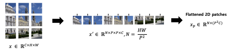
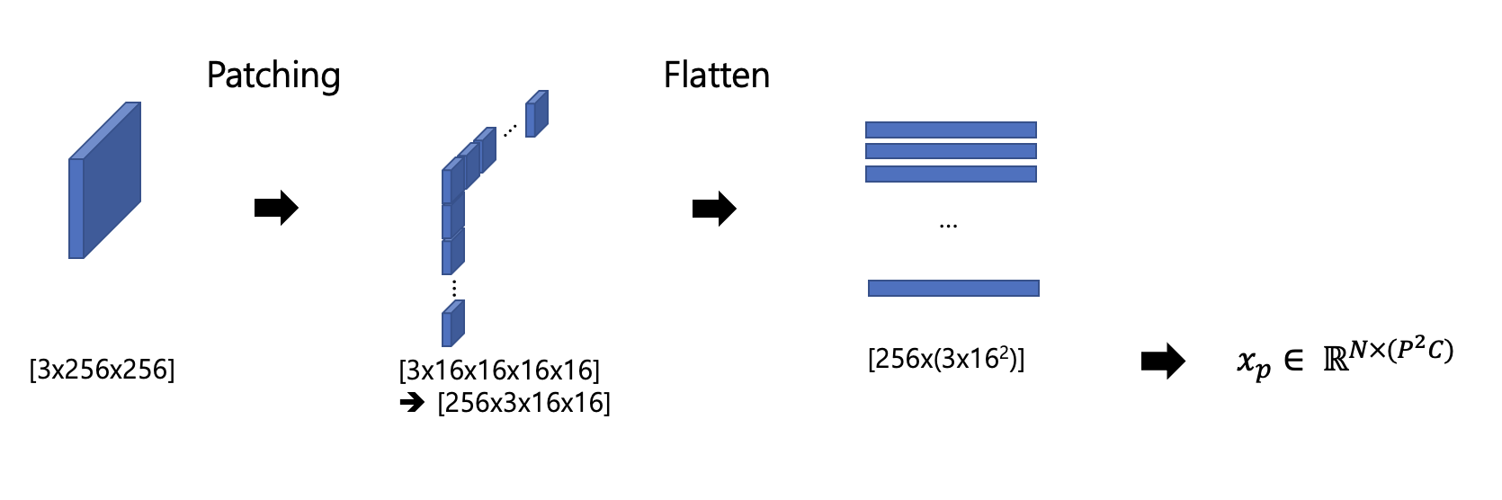
Figure4. Divide the input image into fixed size patches. And flatten each patches to stack as columns. P, N stands for patch size and total number of patches respectively.


C, H, and W represent the number of channels, height and width, respectively. And P represents the size of the patch. Each patch is size of (C, P, P) and N means the total number of patches. The total number of patches N can be obtained through

Linear projection is a process corresponding to the red area above among the entire ViT structure.
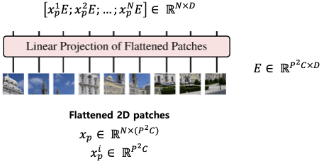
Figure5. Flatten the patches and get it through a linear layer to form a tensor of specific size.

- Each flattened 2d patch is multiplied by E, which is a Linear Projection Matrix, and the vector size is changed to a latent vector size (D).
- The shape of E becomes (
$P^2C, D$ ), and when$x_p$ is multiplied by E, it has the size (N, D). If the batch size is also considered, a tensor having a size of (B, N, D) can be finally obtained.
Like BERT(arXiv, PDF), transformer trains class token by passing it through multiple encoder blocks. The class token first initialized with zeros and appended to the input. Just like BERT, the NLP transformer also uses class token. Consequently, class token was inherited to vision transformer too. On vision transformer. The class token is a special symbol to train. Even if it looks like a part of the input, as long as it's a trainable parameter, it make more sense to treat it as a part of the model.

Positional embedding is a process corresponding to the red area above among the entire ViT structure.
First, you should understand that sequence is a kind of position. The authors of NLP transformer tried to embed fixed positional values to the input and the value was formulated as ${p_t}^{(i)} := \begin{cases} \sin(w_k \bullet t) \quad \mathrm{if} i=2k \ \cos(w_k \bullet t) \quad \mathrm{if} i=2k+1 \ \end{cases}, w_t = {1 \over {10000^{2k/d}}}$. This represents unique positional information to all tokens. On the other hand, vision transformer, set the positional information as another learnable parameter.
Figure6. Add the class token to the embedding result as shown in the figure above. Then a matrix of size (N, D) becomes of size (N+1, D).

- Add CLS Token, a learnable random vector of 1xD size.
- Add
$E_{pos}$ , a learnable random vector of size (N+1)xD. - The final Transformer input becomes
$z_0$ .
After the training, the positional vector is looks like Figure7.
Figure7. Position embeddings of models trained with different hyperparameters.

They applied GELU activation function(arXiv, PDF) proposed by Dan Hendrycks and Kevin Gimpel. They combined dropout, zoneout and ReLU activation function to formulate GELU. ReLU gives non-linearity by dropping negative outputs and os as GELU. Let
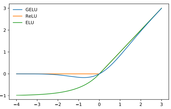
Figure8. Graph comparison among GELU, ReLU and ELU activation functions.

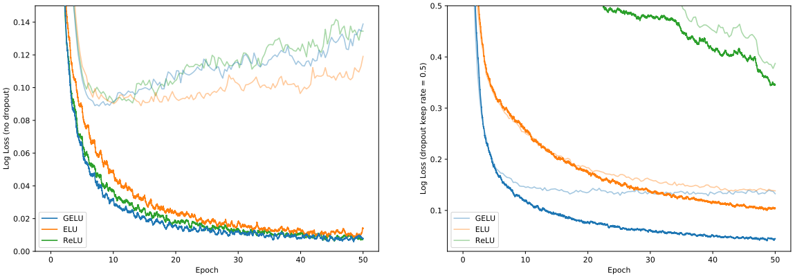
Figure9. MNIST Classification Results. Left are the loss curves without dropout, and right are curves with a dropout rate of 0.5. Each curve is the the median of five runs. Training set log losses are the darker, lower curves, and the fainter, upper curves are the validation set log loss curves.

See the paper for more experiments.

Layer normalization is a stage to normalize the features of pixels and channels for one sample.
This normalization is sample independent and normalizes the total image tensor.
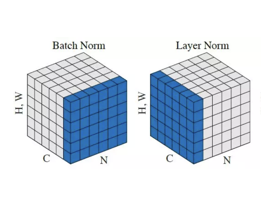
Figure10. Comparison of normalization target between batch normalization and layer normalization.

- Batch Normalization operates only on N, H, and W. Therefore, the mean and standard deviation are calculated regardless of channel map C and normalized for batch N.
- Since Layer Normalization operates only on C, H, W, the mean and standard deviation are calculated regardless of batch N. That is, it is normalized to channel map C.
- Layer normalization is more used than batch normalization because the mini-batch length can be different in NLP's Transformer. ViT borrowed NLP's Transformer Layner normalization.