The source code is to be found in the root directory. In the directory Release, you will find the makefile and a script for running on the EPFL cluster.
The main optimized version of the parallelized Conjugate-Gradient solver for PSD matrices is implemented in CUDA C/C++. A sequential version implemented in C is also available to compare the results of the CUDA implementation.
Most of the kernels have optimal intuitive implementation like the vector-vector additionkernel or the scalar-vector multiplication kernel. These kernels will therefore not be discussedand we will focus on the 2 main kernels of this algorithm namely, the matrix-vector product and the vector-vector inner product.
A lot of different kernels can be written for this one seemingly simple task with coalesced memory access, usage of shared-memory and no bank conflict. The implemented version takes advantage of the fact that the system matrix A is a PSD symmetric matrix. For further description of the kernel, assume that the matrix A is of dimension SIZE x SIZE.
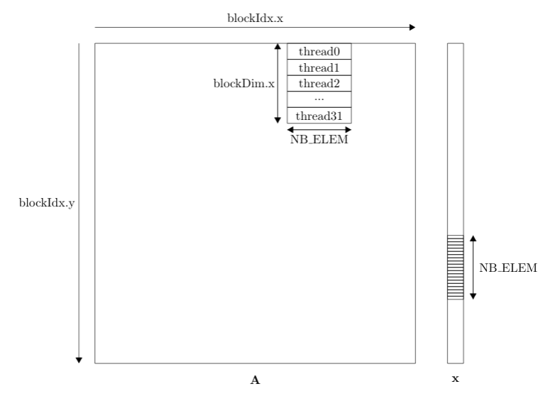
First of all, let us define the grid and block dimensions. The kernel is launched with a 2D grid and 1D blocks. This is schematically illustrated in the figure below. In short, a) each individual thread computes a vector-vector inner product of size NB_ELEM. Then b) this inner product is added to the corresponding position in the output vector.
Within a block, every threads access the same elements of the vector x. Therefore, a corresponding section of the vector x is loaded into shared memory at the beginning of the kernel for faster memory access. Every thread then iterates over the elements in shared memory to compute the inner product with a section of the corresponding row of A. However, accessing elements of A in this manner is sub-optimal since it is not a coalesced memory access. This has to do with the way threads are mapped on the underlying hardware in warps. Global memory is accessed via 32-, 64-, or 128-byte memory transactions. Threads are mapped in warps sequentially based on their thread ID. Therefore, threads accessing memory in a non coalesced fashion will generate a 32-byte memory transaction for a single float of 4 bytes reducing the throughput by a factor of 8.
However an easy solution for only generating 128-byte memory transaction is to access the transposed element. Transposed elements are the same since our matrix A is symmetric. This solution applies to row-major stored matrices. If the matrix was col-major stored, there would not have been any issue in the first place and accessing the transposed element would result in a non-coalesced memory access.
It is also worth pointing out that iterating over the elements stored in shared memory won't result in a bank conflict. Since each thread accesses the same element at every iteration, there will be a broadcast.
The second part of the kernel consists of adding the inner product of each thread to the corresponding position in the output vector. This is done using the atomicAdd() function. Atomic functions are functions that perform a read-operation-write at some position in memory by certifying that there will not be any interference from other threads.
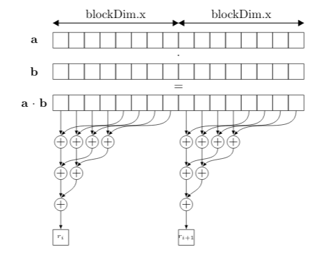
This kernel uses a 1D grid as well as 1D blocks. This is schematically illustrated in the figure below. In short each block computes a smaller vector-vector inner product and all these reductions are added together at the output memory location in an atomic manner.
Each block accesses vectors a and b in a coalesced fashion and each thread within the blocks loads a subsection of the element-wise product of a and b into shared memory. Then a reduction of the elements in shared memory takes place. Such a reduction is not cannot be fully parallelized since every element has to be added with every other elements.
After all blocks have their partial reduced value, we still need to reduce all of these values. This is simply done using the atomicAdd() function. Note that we could store all the partial sums in a vector and reduce it in a new kernel in the same manner. This was implemented and was shown to be about 10% slower with all the added overhead.
The dimension of the grid and of the blocks have not thoroughly discussed. The optimal block size are in fact strongly dependent on the size of the problem and on the underlying hardware. The best way to find these optimal sizes are to grid search for each size of the problem and for each targeted hardware. A good rule of thumb applied for this implementation is to have block sizes that are multiple of 32 to insure complete warps. Depending on the kernel, it is also worth noting that the block size should not be too big to be able to store the corresponding memory chunks in shared memory.
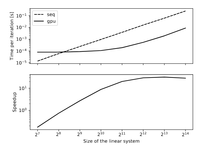
Multiple runs of both the sequential and the CUDA version have been run for different sizes of the problem on the EPFL cluster. The results are graphically shown in the figure below. The running times have been normalized by the number of iteration to prevent the condition number of the generated matrices to have an impact on the performance. We obtained a speedup of 30 for large problem sizes.
The results are intuitively understandable. It is worth noting that the figure is plotted on a loglog scale. The sequential version behaves as expected. An iteration of the algorithm is essentially a couple of vector addition / inner product which have a linear algorithmic but also a matrix-vector product with a quadratic algorithmic complexity. Therefore, running one iteration with a size twice as big should lead to a running time 4 times as large. A starting size of 128 is large enough for the sequential curve to be quadratic on the whole span of the graph. On the other hand, the CUDA version only behave in the same manner for large problems sizes. This has to do with the fact that the GPU has 2880 CUDA cores, most of which are idle for small problem sizes. Increasing the problem size from 2^7 to 2^9 has almost no impact on the running time of a single iteration. This corresponds to less and less CUDA cores being idle but the number of launched warps stays roughly the same. For large problem sizes, the slope of the 2 curves are the same and the curves run parallel. The speedup curve is simply obtained as the ratio of the seq and the gpu curve.
These results show that it is more advantageous to run the CG algorithm on CPU for small problem sizes. For very small problem sizes, the gpu version is orders of magnitude slower. Moreover, the performance curves don't take into account the latency of the memory transfers between the host and the device. For a decent number of iteration, this latency is not noticeable but for matrices with low condition number, it could be worth taking that into account as well.


