mottelet / Polynomials.jl

Polynomial manipulations in Julia

Polynomials.jl

Basic arithmetic, integration, differentiation, evaluation, and root finding over dense univariate polynomials.

Installation

(v1.6) pkg> add Polynomials

Available Types of Polynomials

• Polynomial –⁠ standard basis polynomials, a(x) = a₀ + a₁ x + a₂ x² + … + aₙ xⁿ, n ∈ ℕ
• ImmutablePolynomial –⁠ standard basis polynomials backed by a Tuple type for faster evaluation of values
• SparsePolynomial –⁠ standard basis polynomial backed by a dictionary to hold sparse high-degree polynomials
• LaurentPolynomial –⁠ Laurent polynomials, a(x) = aₘ xᵐ + … + aₙ xⁿ m ≤ n, m,n ∈ ℤ backed by an offset array; for example, if m<0 and n>0, a(x) = aₘ xᵐ + … + a₋₁ x⁻¹ + a₀ + a₁ x + … + aₙ xⁿ
• FactoredPolynomial –⁠ standard basis polynomials, storing the roots, with multiplicity, and leading coefficient of a polynomial
• ChebyshevT –⁠ Chebyshev polynomials of the first kind
• RationalFunction - a type for ratios of polynomials.

Usage

julia> using Polynomials

Construction and Evaluation

Construct a polynomial from an array (a vector) of its coefficients, lowest order first.

julia> Polynomial([1,0,3,4])
Polynomial(1 + 3*x^2 + 4*x^3)

Optionally, the variable of the polynomial can be specified.

julia> Polynomial([1,2,3], :s)
Polynomial(1 + 2*s + 3*s^2)

Construct a polynomial from its roots.

julia> fromroots([1,2,3]) # (x-1)*(x-2)*(x-3)
Polynomial(-6 + 11*x - 6*x^2 + x^3)

Evaluate the polynomial p at x.

julia> p = Polynomial([1, 0, -1]);
julia> p(0.1)
0.99

Arithmetic

Methods are added to the usual arithmetic operators so that they work on polynomials, and combinations of polynomials and scalars.

julia> p = Polynomial([1,2])
Polynomial(1 + 2*x)

julia> q = Polynomial([1, 0, -1])
Polynomial(1 - x^2)

julia> p - q
Polynomial(2*x + x^2)

julia> p = Polynomial([1,2])
Polynomial(1 + 2*x)

julia> q = Polynomial([1, 0, -1])
Polynomial(1 - x^2)

julia> 2p
Polynomial(2 + 4*x)

julia> 2+p
Polynomial(3 + 2*x)

julia> p - q
Polynomial(2*x + x^2)

julia> p * q
Polynomial(1 + 2*x - x^2 - 2*x^3)

julia> q / 2
Polynomial(0.5 - 0.5*x^2)

julia> q ÷ p # `div`, also `rem` and `divrem`
Polynomial(0.25 - 0.5*x)

Operations involving polynomials with different variables will error.

julia> p = Polynomial([1, 2, 3], :x);
julia> q = Polynomial([1, 2, 3], :s);
julia> p + q
ERROR: ArgumentError: Polynomials have different indeterminates

Construction and Evaluation

While polynomials of type Polynomial are mutable objects, operations such as +, -, *, always create new polynomials without modifying its arguments. The time needed for these allocations and copies of the polynomial coefficients may be noticeable in some use cases. This is amplified when the coefficients are for instance BigInt or BigFloat which are mutable themself. This can be avoided by modifying existing polynomials to contain the result of the operation using the MutableArithmetics (MA) API. Consider for instance the following arrays of polynomials

using Polynomials
d, m, n = 30, 20, 20
p(d) = Polynomial(big.(1:d))
A = [p(d) for i in 1:m, j in 1:n]
b = [p(d) for i in 1:n]

In this case, the arrays are mutable objects for which the elements are mutable polynomials which have mutable coefficients (BigInts). These three nested levels of mutable objects communicate with the MA API in order to reduce allocation. Calling A * b requires approximately 40 MiB due to 2 M allocations as it does not exploit any mutability. Using

using MutableArithmetics
const MA = MutableArithmetics
MA.operate(*, A, b)

exploits the mutability and hence only allocate approximately 70 KiB due to 4 k allocations. If the resulting vector is already allocated, e.g.,

z(d) = Polynomial([zero(BigInt) for i in 1:d])
c = [z(2d - 1) for i in 1:m]

then we can exploit its mutability with

MA.mutable_operate!(MA.add_mul, c, A, b)

to reduce the allocation down to 48 bytes due to 3 allocations. These remaining allocations are due to the BigInt buffer used to store the result of intermediate multiplications. This buffer can be preallocated with

buffer = MA.buffer_for(MA.add_mul, typeof(c), typeof(A), typeof(b))
MA.mutable_buffered_operate!(buffer, MA.add_mul, c, A, b)

then the second line is allocation-free.

The MA.@rewrite macro rewrite an expression into an equivalent code that exploit the mutability of the intermediate results. For instance

MA.@rewrite(A1 * b1 + A2 * b2)

is rewritten into

c = MA.operate!(MA.add_mul, MA.Zero(), A1, b1)
MA.operate!(MA.add_mul, c, A2, b2)

which is equivalent to

c = MA.operate(*, A1, b1)
MA.mutable_operate!(MA.add_mul, c, A2, b2)

Note that currently, only the Polynomial implements the API and it only implements part of it.

Integrals and Derivatives

Integrate the polynomial p term by term, optionally adding a constant term k. The degree of the resulting polynomial is one higher than the degree of p (for a nonzero polynomial).

julia> integrate(Polynomial([1, 0, -1]))
Polynomial(1.0*x - 0.3333333333333333*x^3)

julia> integrate(Polynomial([1, 0, -1]), 2)
Polynomial(2.0 + 1.0*x - 0.3333333333333333*x^3)

Differentiate the polynomial p term by term. The degree of the resulting polynomial is one lower than the degree of p.

julia> derivative(Polynomial([1, 3, -1]))
Polynomial(3 - 2*x)

Root-finding

Return the roots (zeros) of p, with multiplicity. The number of roots returned is equal to the degree of p. By design, this is not type-stable, the returned roots may be real or complex.

julia> roots(Polynomial([1, 0, -1]))
2-element Vector{Float64}:
 -1.0
  1.0

julia> roots(Polynomial([1, 0, 1]))
2-element Vector{ComplexF64}:
 0.0 - 1.0im
 0.0 + 1.0im

julia> roots(Polynomial([0, 0, 1]))
2-element Vector{Float64}:
 0.0
 0.0

Fitting arbitrary data

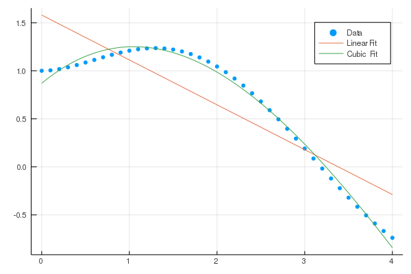
Fit a polynomial (of degree deg or less) to x and y using a least-squares approximation.

julia> xs = 0:4; ys = @. exp(-xs) + sin(xs);

julia> fit(xs, ys) |> p -> round.(coeffs(p), digits=4) |> Polynomial
Polynomial(1.0 + 0.0593*x + 0.3959*x^2 - 0.2846*x^3 + 0.0387*x^4)

julia> fit(ChebyshevT, xs, ys, 2) |> p -> round.(coeffs(p), digits=4) |> ChebyshevT
ChebyshevT(0.5413⋅T_0(x) - 0.8991⋅T_1(x) - 0.4238⋅T_2(x))

Visual example:

Other methods

Polynomial objects also have other methods:

• 0-based indexing is used to extract the coefficients of [a0, a1, a2, ...], coefficients may be changed using indexing notation.

• coeffs: returns the entire coefficient vector

• degree: returns the polynomial degree, length is number of stored coefficients

• variable: returns the polynomial symbol as polynomial in the underlying type

• norm: find the p-norm of a polynomial

• conj: finds the conjugate of a polynomial over a complex field

• truncate: set to 0 all small terms in a polynomial;

• chop chops off any small leading values that may arise due to floating point operations.

• gcd: greatest common divisor of two polynomials.

• Pade: Return the Pade approximant of order m/n for a polynomial as a Pade object.

Related Packages

• StaticUnivariatePolynomials.jl Fixed-size univariate polynomials backed by a Tuple

• MultiPoly.jl for sparse multivariate polynomials

• DynamicPolynomals.jl Multivariate polynomials implementation of commutative and non-commutative variables

• MultivariatePolynomials.jl for multivariate polynomials and moments of commutative or non-commutative variables

• PolynomialRings.jl A library for arithmetic and algebra with multi-variable polynomials.

• AbstractAlgebra.jl, Nemo.jl for generic polynomial rings, matrix spaces, fraction fields, residue rings, power series, Hecke.jl for algebraic number theory.

• CommutativeAlgebra.jl the start of a computer algebra system specialized to discrete calculations with support for polynomials.

• PolynomialRoots.jl for a fast complex polynomial root finder. For larger degree problems, also FastPolynomialRoots and AMRVW.

• SpecialPolynomials.jl A package providing various polynomial types beyond the standard basis polynomials in Polynomials.jl. Includes interpolating polynomials, Bernstein polynomials, and classical orthogonal polynomials.

• ClassicalOrthogonalPolynomials.jl A Julia package for classical orthogonal polynomials and expansions. Includes chebyshevt, chebyshevu, legendrep, jacobip, ultrasphericalc, hermiteh, and laguerrel. The same repository includes FastGaussQuadrature.jl, FastTransforms.jl, and the ApproxFun packages.

Legacy code

As of v0.7, the internals of this package were greatly generalized and new types and method names were introduced. For compatability purposes, legacy code can be run after issuing using Polynomials.PolyCompat.

Contributing

If you are interested in contributing, feel free to open an issue or pull request to get started.