Steganalysis, a critical discipline within cybersecurity, is dedicated to uncovering hidden information concealed within digital media. In this specific implementation, Support Vector Machines (SVM) are employed for steganalysis, with a focus on binary classification between cover and stego images.
-
Terrorism:
Steganography, the technique of hiding information within digital media, has raised concerns regarding its potential misuse in various cybersecurity scenarios. The low detection risk associated with steganography prompts the exploration of steganalysis to mitigate risks such as terrorism, espionage, and hacking.
-
Espionage:
Steganography serves as a covert communication method for passing messages through public platforms. Notably, instances like the use of steganography by individuals such as Anna Chapman and her espionage ring highlight the need for robust steganalysis techniques.
-
Hacking:
The concealment of malicious code within images or audio files through steganography poses a threat in hacking scenarios. The ability to hide executable code within innocuous files presents challenges for traditional detection methods, necessitating advanced steganalysis approaches.
The steganalysis process involves two main phases: feature extraction and classification. Features are extracted from images, and SVM classifiers are trained to distinguish between cover and stego classes.

In the defineData function, the process of converting images to vectors serves multiple purposes in the context of steganalysis:
-
Spatial Information Representation: Images are inherently structured in a two-dimensional grid of pixels. Converting them to vectors flattens this structure, representing each pixel's intensity as an element in the vector. This transformation allows the preservation of spatial information while making it suitable for machine learning algorithms.
-
Uniform Input Format: By converting images to vectors, we achieve a uniform input format for SVM training. SVMs require consistent input dimensions, and transforming images into vectors ensures that each sample has the same length, facilitating the learning process.
-
Dimensionality Reduction: While images are typically high-dimensional, converting them to vectors performs a form of dimensionality reduction. This simplification helps in speeding up the training process and can be beneficial when dealing with large datasets.
The normalization step ensures that pixel intensities, which typically range from 0 to 255, are scaled to a standard range (0 to 1). Normalization is essential for maintaining numerical stability during the training of machine learning models. It prevents features with larger magnitudes from dominating the learning process, ensuring that all features contribute equally to the model.
-
Support Vectors: SVM operates by identifying support vectors, which are the data points that influence the position of the hyperplane. These vectors play a crucial role in determining the optimal decision boundary.
-
Maximizing Margin: The SVM algorithm seeks to find the hyperplane that maximizes the margin, i.e., the distance between the hyperplane and the closest data points from each class. A larger margin enhances the model's generalization to unseen data.
-
Linear Kernel (Default): The linear kernel creates a straight hyperplane, suitable for linearly separable data. It forms the baseline for comparison with other kernels.
-
Non-Linear Kernels: Polynomial and radial basis function (RBF) kernels introduce non-linearity to the decision boundary. They enable SVM to handle more complex relationships within the data.
In the implementation, a linear kernel is initially chosen. Experimentation with alternative kernels, such as polynomial or RBF, allows observation of the impact on the decision boundaries and, consequently, the classification accuracy.
-
Polynomial Kernel: A polynomial kernel introduces higher-order terms, enabling the SVM to capture non-linear relationships. The degree of the polynomial determines the complexity of the decision boundary.
-
RBF Kernel: The radial basis function (RBF) kernel is versatile and can model complex decision boundaries. It considers the similarity between data points in a high-dimensional space.
-
Hyperparameter Tuning: Adjusting hyperparameters, such as the degree of the polynomial kernel or the gamma value for the RBF kernel, can further optimize SVM performance.
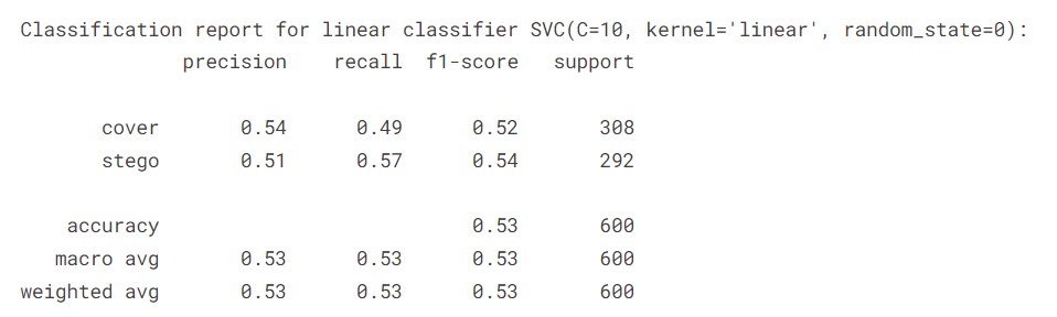
The classification report and confusion matrix obtained after testing with different kernels provide a comprehensive assessment of each kernel's performance. Metrics such as precision, recall, and F1-score shed light on the classifier's ability to correctly classify cover and stego images.
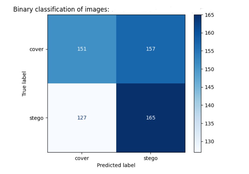
The graphical representation of the confusion matrix allows for a visual understanding of how well the SVM model distinguishes between the two classes under different kernels. This experimentation aids in selecting the most suitable kernel for the specific steganalysis task at hand.
# Importing necessary libraries
from sklearn import svm, metrics
from sklearn.metrics import ConfusionMatrixDisplay
from sklearn.model_selection import train_test_split
from sklearn.preprocessing import StandardScaler

import matplotlib.pyplot as plt
from skimage import io, transform
import numpy as np
import time
import os

# Function to collect images and labels
def collectImages(image_paths, images, labels, label):
    for image_path in image_paths:
        image = io.imread(image_path)
        images.append(image)
        labels.append(label)

# Function to define and preprocess data
def defineData():
    class_size = 1000  # Size of each class

    images = []       # List to store images
    labels = []       # List to store labels

    # Define paths for cover images
    image_paths_cover = [dataset_dir + "/Cover/" + image_path for image_path in os.listdir(dataset_dir + "/Cover/") if image_path.endswith(".jpg")][: class_size]
    collectImages(image_paths_cover, images, labels, "cover")

    # Define paths for stego images
    image_paths_stego = [dataset_dir + "/Stego/" + image_path for image_path in os.listdir(dataset_dir + "/Stego/") if image_path.endswith(".jpg")][: class_size]
    collectImages(image_paths_stego, images, labels, "stego")

    images = np.array(images)
    labels = np.array(labels)

    n_samples = len(images)

    # Convert to vector
    data = images.reshape((n_samples, -1))
    print("\nVector shape:")
    print(data.shape)

    # Normalize data
    data = data / 255.0

    return data, labels

# Function to create SVM classifier
def create_svc(kernel_in, data, labels):
    X_train, X_test, y_train, y_test = train_test_split(data, labels, random_state=0, test_size=0.3, shuffle=True)
    X_train = X_train ** 2

    # Creating SVM classifier
    if kernel_in == 'linear':
        classifier = svm.SVC(kernel=kernel_in, C=10, random_state=0)
    elif kernel_in == 'poly':
        classifier = svm.SVC(kernel=kernel_in, C=10, random_state=0, degree=2, gamma='auto')
    else:
        sc = StandardScaler()
        X_train = sc.fit_transform(X_train)
        X_test = sc.fit_transform(X_test)
        classifier = svm.SVC(kernel=kernel_in, C=1000, random_state=1234, gamma='auto')

    # Fitting the SVM classifier
    model = classifier.fit(X=X_train, y=y_train)

    # Making predictions
    prediction = classifier.predict(X_test)

    # Displaying classification report and confusion matrix
    print("Classification report for linear classifier %s:\n%s\n"
          % (classifier, metrics.classification_report(y_test, prediction)))

    np.set_printoptions(precision=2)
    disp = ConfusionMatrixDisplay.from_estimator(
        classifier,
        X_test,
        y_test,
        display_labels=["cover", "stego"],
        cmap=plt.cm.Blues,
        normalize=None,
    )
    disp.ax_.set_title("Binary classification of images: cover vs stego")

    print(disp.confusion_matrix)
    plt.show()

    return model, classifier, prediction

# Main execution
gc.collect()
dataset_dir = "/kaggle/input/alaska2-image-steganalysis"

start_time = time.time()

# Define and preprocess data
data, labels = defineData()

# Create SVM classifier
create_svc('linear', data, labels)

print(f"Total time taken: {(time.time() - start_time):.2f} seconds")The provided Python code implements a steganalysis approach using Support Vector Machines (SVM) for binary classification between cover and stego images. This section offers a detailed explanation of the code's various components, emphasizing the key aspects of data processing, SVM classification, and the evaluation of different kernels.
The defineData function initiates the process by collecting images from the "Cover" and "Stego" directories. Each image is then labeled accordingly, designating it as either "cover" or "stego." The pivotal step of converting these images into vectors is undertaken, transforming the inherent spatial information into a format suitable for SVM training. Normalization follows, ensuring consistent input ranges and preventing numerical instabilities during the learning process.
The heart of the steganalysis lies in SVM classification, and the create_svc function orchestrates this phase. Initially opting for a linear kernel, the SVM is trained on the squared training set. Support vectors, pivotal in defining the optimal hyperplane, are identified, and the algorithm aims to maximize the margin between different classes. The decision boundary, in the case of a linear kernel, is a straight line.
The code goes beyond a singular kernel choice, allowing for experimentation with various alternatives. Polynomial and radial basis function (RBF) kernels are introduced to capture non-linear relationships within the data. The degree of the polynomial and the gamma parameter for the RBF kernel are crucial hyperparameters that influence the shape and complexity of the decision boundary.
The evaluation metrics, including precision, recall, and F1-score, provide detailed insights into the performance of the SVM classifier under different kernels. The confusion matrix, graphically displayed, aids in comprehending how well the model distinguishes between cover and stego images. By comparing the results obtained with distinct kernels, the steganalysis efficacy is thoroughly examined, facilitating an informed decision on the most suitable kernel for the specific dataset.
The code is structured to facilitate modularity and reusability. Functions such as collectImages, defineData, and create_svc encapsulate specific functionalities, promoting clarity and ease of maintenance. The utilization of libraries such as scikit-learn enhances code efficiency, providing a robust foundation for SVM implementation.
The implementation encourages further exploration and experimentation. Researchers and practitioners can delve into hyperparameter tuning, potentially improving the SVM's performance under various scenarios. Additionally, the code serves as a baseline for extending steganalysis techniques, potentially incorporating advanced feature extraction methods or exploring alternative machine learning algorithms.
In conclusion, the code presents a comprehensive steganalysis methodology leveraging SVM classification. From data preprocessing to SVM training and kernel evaluation, each step is meticulously implemented and explained. The modularity of the code allows for easy adaptation and experimentation, making it a valuable resource for researchers and practitioners in the field of cybersecurity.