This document generates a visualization of rankings of Metroidvania games according to data from this post on r/metroidvania. It corrects the scores of each game based on the number of people who rated it using an empirical Bayes approach.
Libraries we’ll need:
library(googlesheets4)
library(fitdistrplus)
library(distributional)
library(ggdist)
library(dplyr)
library(rlang)
library(janitor)
library(ggplot2)

theme_set(theme_ggdist())
Read in the data:
# use the commented-out line to read directly from Google Sheets
# df = googlesheets4::read_sheet("https://docs.google.com/spreadsheets/d/1k_6Ehj9rjS34ARqJScHqr-4r1EyMDULcTkbUV4eLr2U/edit#gid=2060671517") |>
df = readr::read_csv("ratings.csv") |>
  clean_names() |>
  mutate(average = average/10)
## New names:
## Rows: 55 Columns: 10
## ── Column specification
## ──────────────────────────────────────────────────────── Delimiter: "," chr
## (4): GAME, %Rated, % [10], ...9 dbl (5): Num. Ratings, Average, B.Avg, StdDev,
## ...10 lgl (1): ...8
## ℹ Use `spec()` to retrieve the full column specification for this data. ℹ
## Specify the column types or set `show_col_types = FALSE` to quiet this message.
## • `` -> `...8`
## • `` -> `...9`
## • `` -> `...10`
Let’s do empirical Bayes to adjust scores based on number of ratings. First we need a prior for the average score based on the distribution of raw averages, which will get by fitting a Beta distribution to the average score (rescaled to be between 0 and 1):
grand_mean_params = fitdist(df$average, "beta")
grand_mean_params
## Fitting of the distribution ' beta ' by maximum likelihood
## Parameters:
## estimate Std. Error
## shape1 19.112474 3.648332
## shape2 6.868662 1.280729
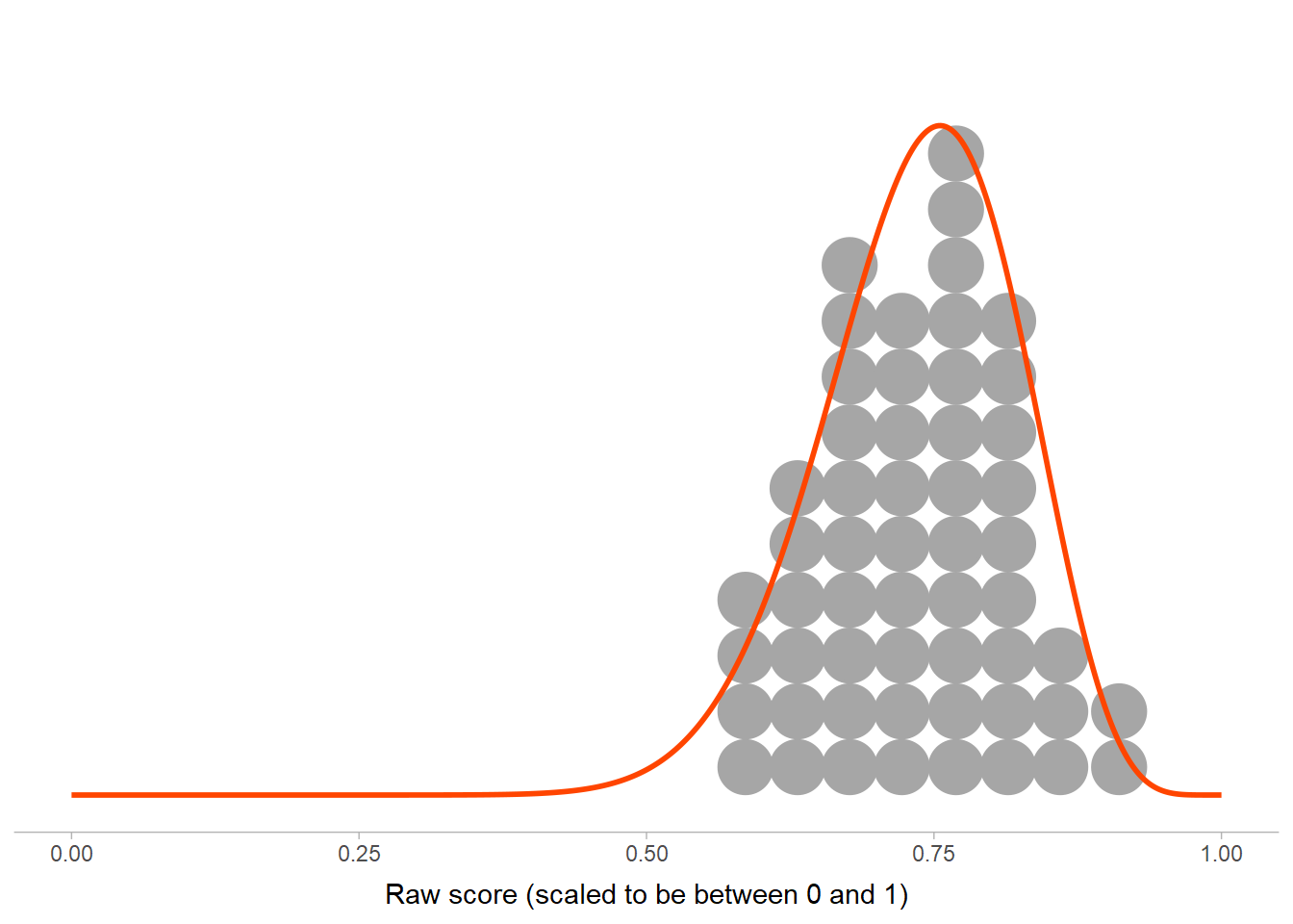
The beta distribution fits the raw scores pretty well:
grand_mean_dist = inject(dist_beta(!!!grand_mean_params$estimate))

ggplot() +
  geom_dots(aes(x = average), data = df) +
  stat_slab(aes(xdist = grand_mean_dist), fill = NA, color = "orangered") +
  scale_y_continuous(breaks = NULL) +
  labs(
    y = NULL,
    x = "Raw score (scaled to be between 0 and 1)"
  ) +
  theme(axis.line.y = element_blank())
To do the adjustment, we consider each rating out of 1 as a fractional “success”; i.e. a rating of 10/10 = 1 by one person is a full “success”, a rating of 0/10 = 0 by one person a full “failure”, and anything else is a fractional “success”. Thus, the existing mean rating on a 0-1 scale can be multiplied by the number of ratings to get the number of “success”es for each game.
To do the empirical Bayes correction, we use the beta distribution above
as a prior on the score of each game. We add the shape1)
parameter to the successes and the shape2) parameter to the
failures, to get new
df_adjusted = df |>
  mutate(
    successes = average * num_ratings,
    failures = num_ratings - successes,
    alpha = successes + grand_mean_params$estimate[["shape1"]],
    beta = failures + grand_mean_params$estimate[["shape2"]],
    average_adjusted = alpha / (alpha + beta),
    rank = rank(-average),
    rank_adjusted = rank(-average_adjusted)
  )
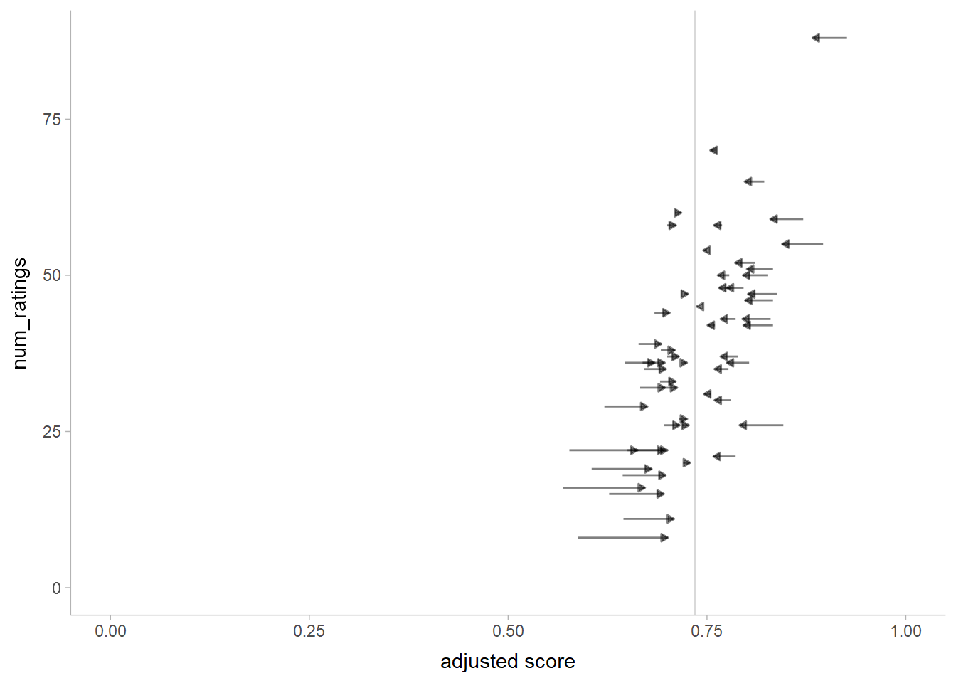
And the adjusted scores are:
df_adjusted |>
  ggplot(aes(y = num_ratings)) +
  geom_vline(xintercept = mean(df$average), color = "gray85") +
  geom_segment(aes(x = average, xend = average_adjusted, yend = num_ratings), arrow = arrow(type = "closed", length = unit(4, "pt")), alpha = 0.5) +
  scale_x_continuous(limits = c(0, 1)) +
  scale_y_continuous(limits = c(0, NA)) +
  labs(x = "adjusted score")
Basically, scores further from the mean are pulled towards it, moreso if they have fewer ratings. This is a conservative adjustment: if we know less about a game (i.e. we have fewer ratings of it), we assume it is closer to the average.
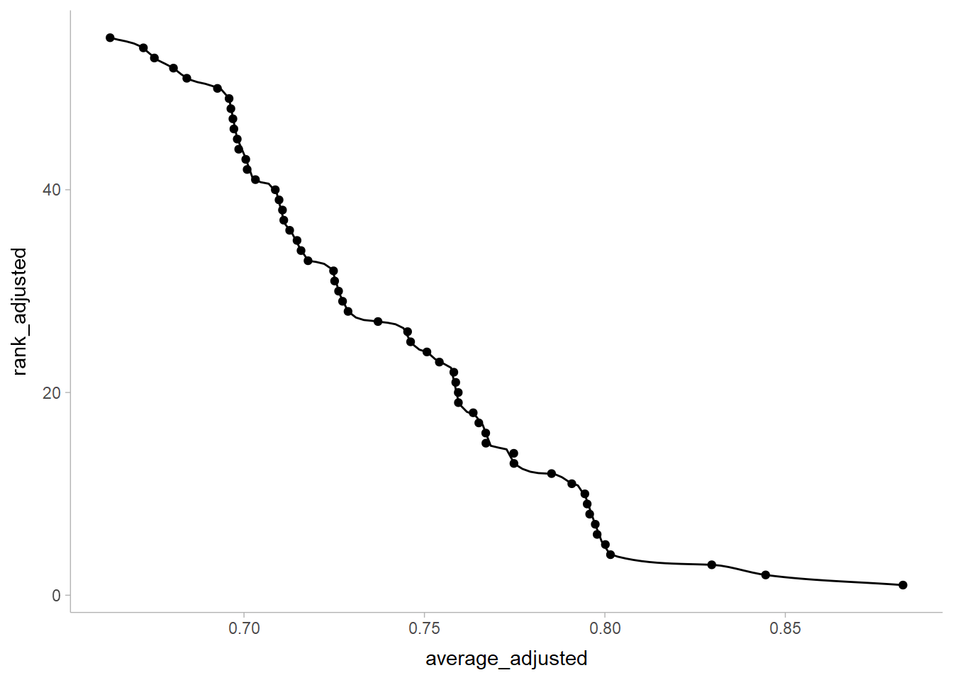
To annotate the plot with ranks and scores, we’ll also need a function from score to approximate rank:
rank_from_average = with(df_adjusted, splinefun(average_adjusted, rank_adjusted, method = "monoH.FC"))

df_adjusted |>
  ggplot(aes(y = rank_adjusted, x = average_adjusted)) +
  stat_function(fun = rank_from_average) +
  geom_point()
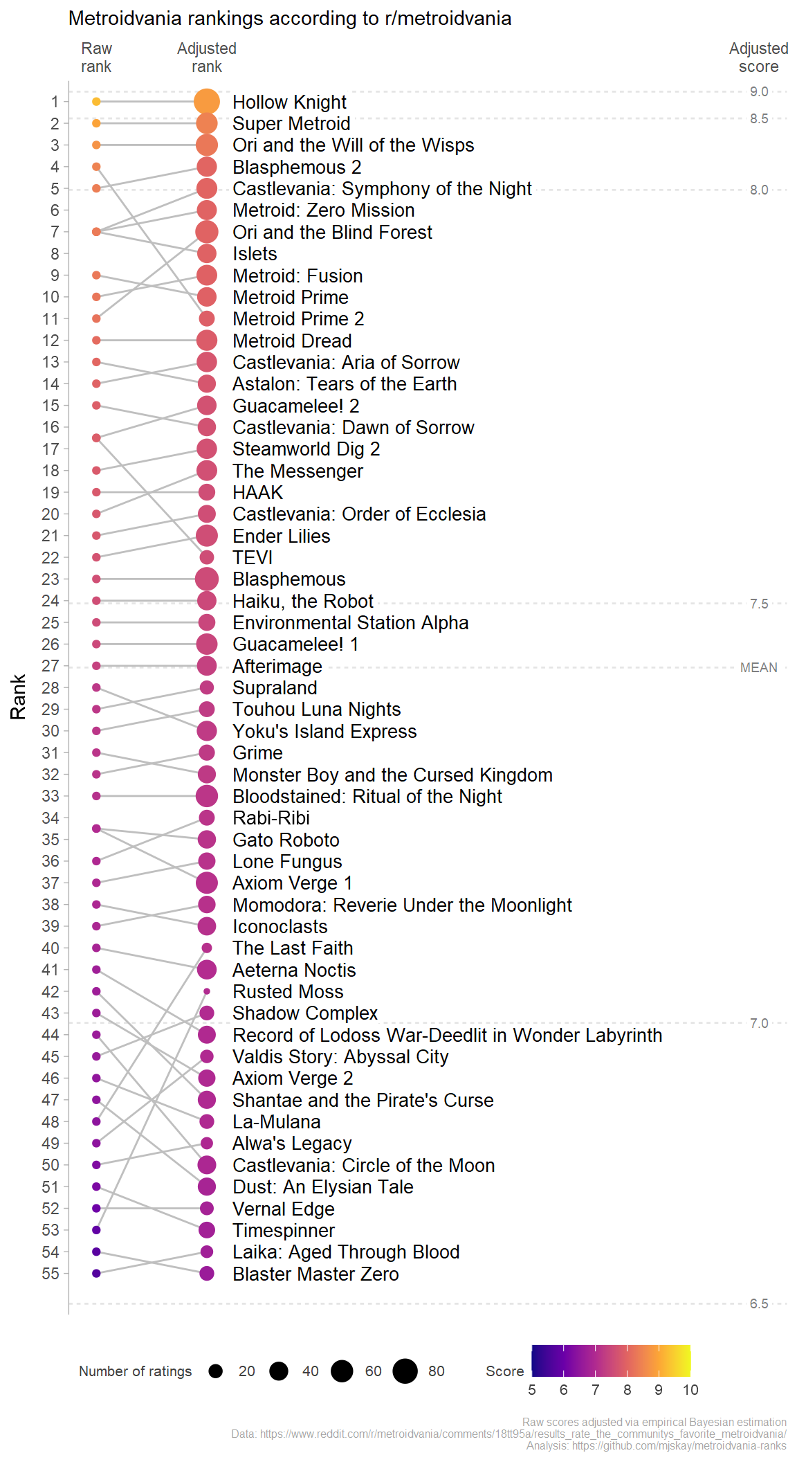
Now we can put together a plot of original ranks/scores and adjusted ranks/scores:
# reference points for scores
average_ref = tibble(
    average = seq(0.65, 0.9, by = 0.05),
    rank = rank_from_average(average),
    label = format(average * 10)
  ) |>
  bind_rows(tibble(
    average = mean(df_adjusted$average),
    rank = rank_from_average(average),
    label = "MEAN"
  ))

df_adjusted |>
  ggplot(aes(y = rank)) +
  geom_hline(aes(yintercept = rank), data = average_ref, color = "gray90", linetype = "22") +
  geom_label(aes(y = rank, label = label), data = average_ref, x = 7, hjust = 0.5, color = "gray50", size = 2.5, label.padding = unit(2, "pt"), label.size = 0) +
  geom_segment(aes(yend = rank_adjusted), x = 1, xend = 2, color = "gray75") +
  geom_point(aes(color = average * 10), x = 1) +
  geom_point(aes(y = rank_adjusted, size = num_ratings, color = average_adjusted * 10), x = 2) +
  geom_label(aes(label = game, y = rank_adjusted), x = 2.2, hjust = 0, size = 3.5, label.padding = unit(2, "pt"), label.size = 0) +
  scale_x_continuous(limits = c(1,7), breaks = c(1,2,7), labels = c("Raw\nrank", "Adjusted\nrank", "Adjusted\nscore"), position = "top", expand = expansion(add = 0.25)) +
  scale_y_reverse(breaks = seq_len(nrow(df_adjusted)), expand = expansion(add = 0.5)) +
  scale_color_viridis_c(limits = c(5,10), option = "plasma") +
  labs(
    x = NULL,
    y = "Rank",
    color = "Score",
    size = "Number of ratings",
    subtitle = "Metroidvania rankings according to r/metroidvania",
    caption = "Raw scores adjusted via empirical Bayesian estimation\nData: https://www.reddit.com/r/metroidvania/comments/18tt95a/results_rate_the_communitys_favorite_metroidvania/\nAnalysis: https://github.com/mjskay/metroidvania-ranks"
  ) +
  theme(
    axis.line.x = element_blank(),
    axis.ticks.x = element_blank(),
    legend.text = element_text(size = 8, color = "gray25"),
    legend.title = element_text(size = 8, color = "gray25", vjust = 0.5),
    legend.title.align = 0,
    legend.box.just = "center",
    legend.position = "bottom",
    legend.justification = 0,
    plot.caption = element_text(size = 6, color = "gray65")
  )


